[1] TRUE14 Trend Analysis
This chapter analyzes temporal trends in consultation volume and the “Consultation Rate” (percentage of total pathology cases that require consultation). Long-term trends in anatomic pathology workload have shown consistent increases in case complexity and volume (Bonert et al. 2021), and digital pathology implementations have been associated with measurable changes in efficiency and consultation patterns (Hanna et al. 2019). Interrupted time series (ITS) analysis is increasingly recognized as the strongest quasi-experimental design for evaluating quality improvement interventions in healthcare, though a systematic review found that 72.5% of published ITS studies had high or very high risk of bias, highlighting the importance of methodological rigor (Hategeka et al. 2020).
14.1 Consultation Rate Over Time
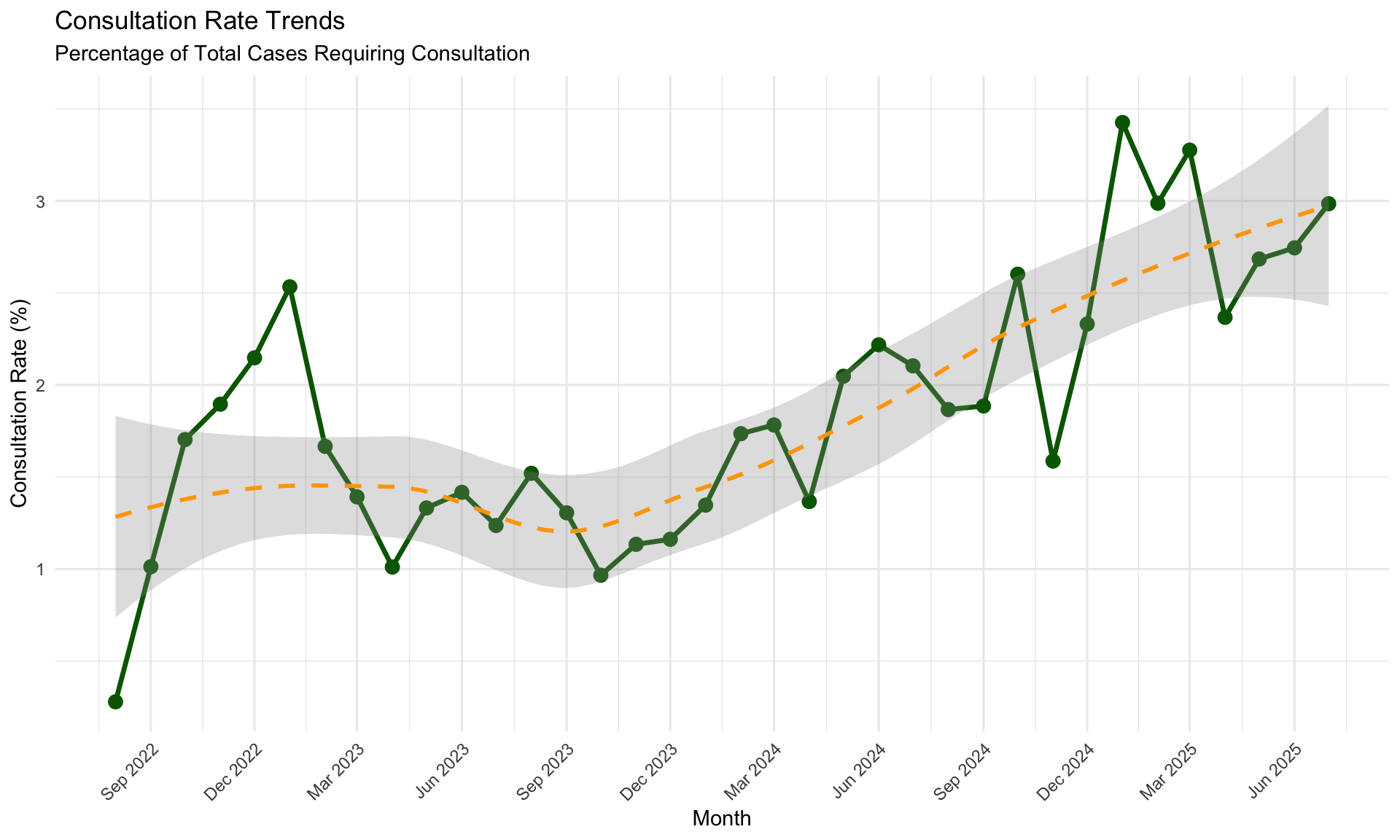
The “Consultation Rate” is defined as the number of internal consultations divided by the total number of pathology cases for the same month.
| Month | Total Cases | Consultations | Rate (%) |
|---|---|---|---|
| 2025-07 | 6298 | 188 | 2.99 |
| 2025-06 | 5136 | 141 | 2.75 |
| 2025-05 | 6593 | 177 | 2.68 |
| 2025-04 | 6082 | 144 | 2.37 |
| 2025-03 | 5494 | 180 | 3.28 |
| 2025-02 | 5690 | 170 | 2.99 |
| 2025-01 | 6129 | 210 | 3.43 |
| 2024-12 | 6005 | 140 | 2.33 |
| 2024-11 | 6113 | 97 | 1.59 |
| 2024-10 | 5611 | 146 | 2.60 |
| 2024-09 | 5567 | 105 | 1.89 |
| 2024-08 | 5892 | 110 | 1.87 |
14.1.1 Monthly Consultation Rate Trend
14.2 Volume Comparison
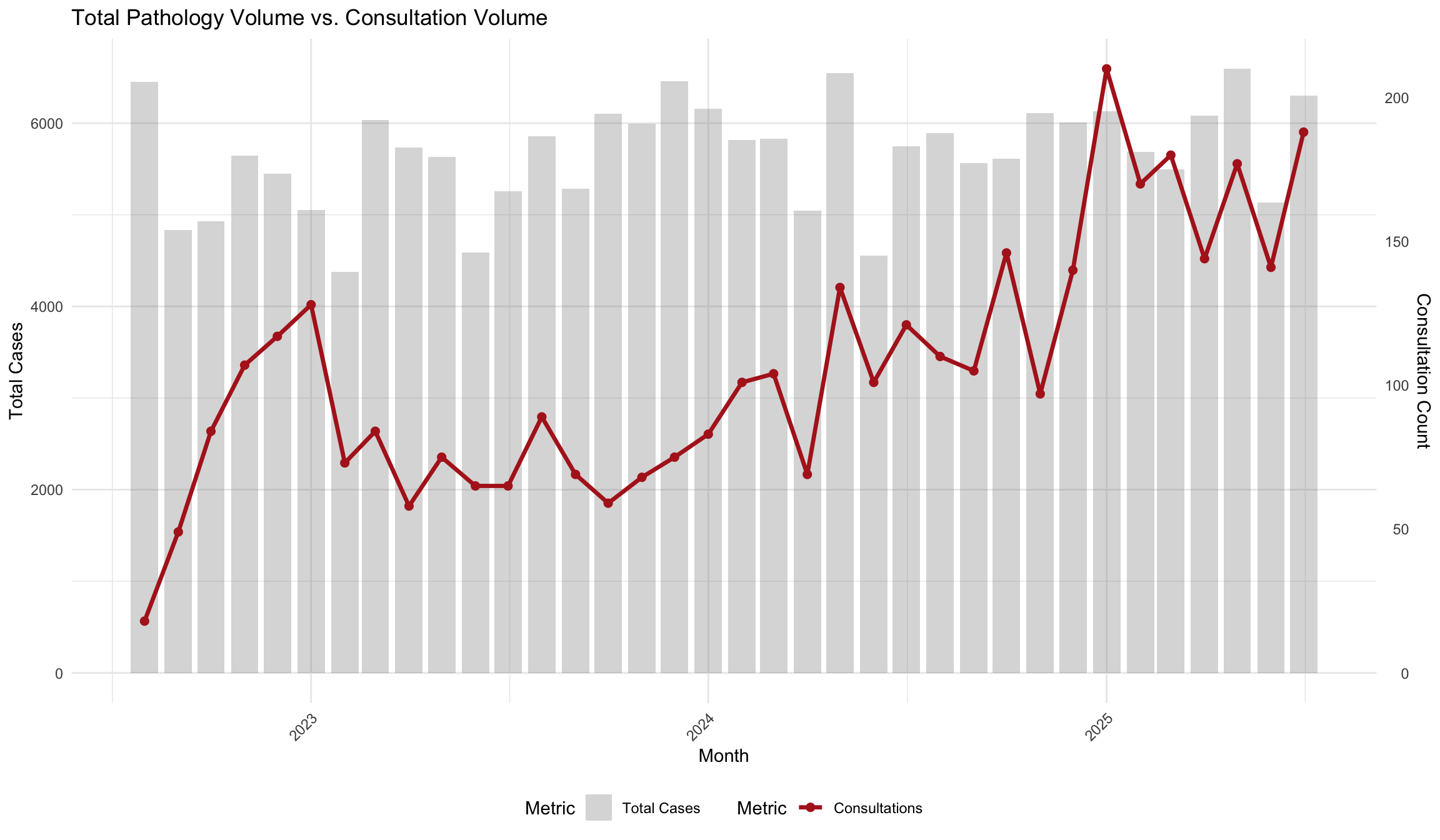
Visualizing the relationship between absolute case volume and consultation requests.
14.3 Subspecialty Trends
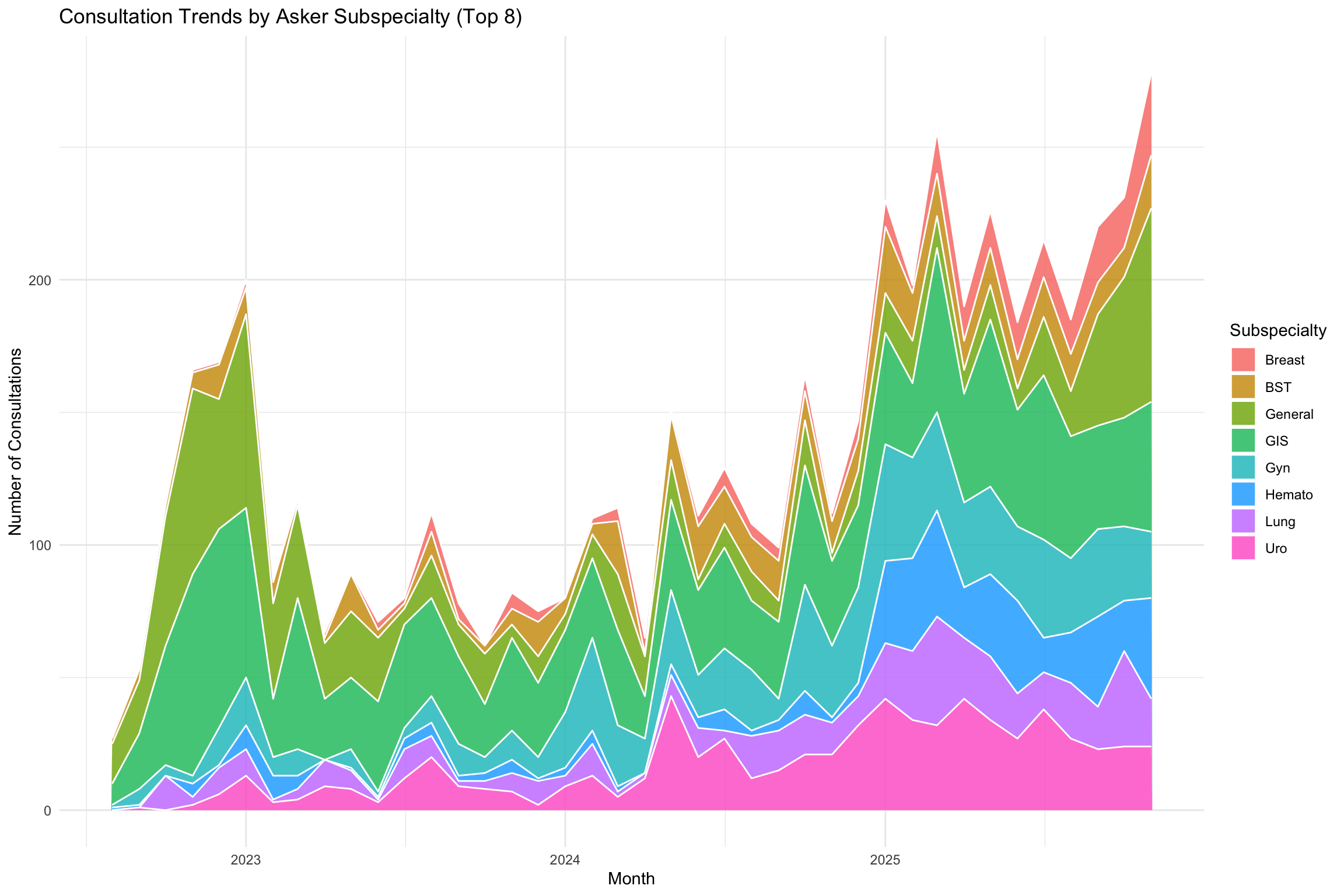
Evolution of consultation topics over time based on the Asker’s 1st subspecialty.
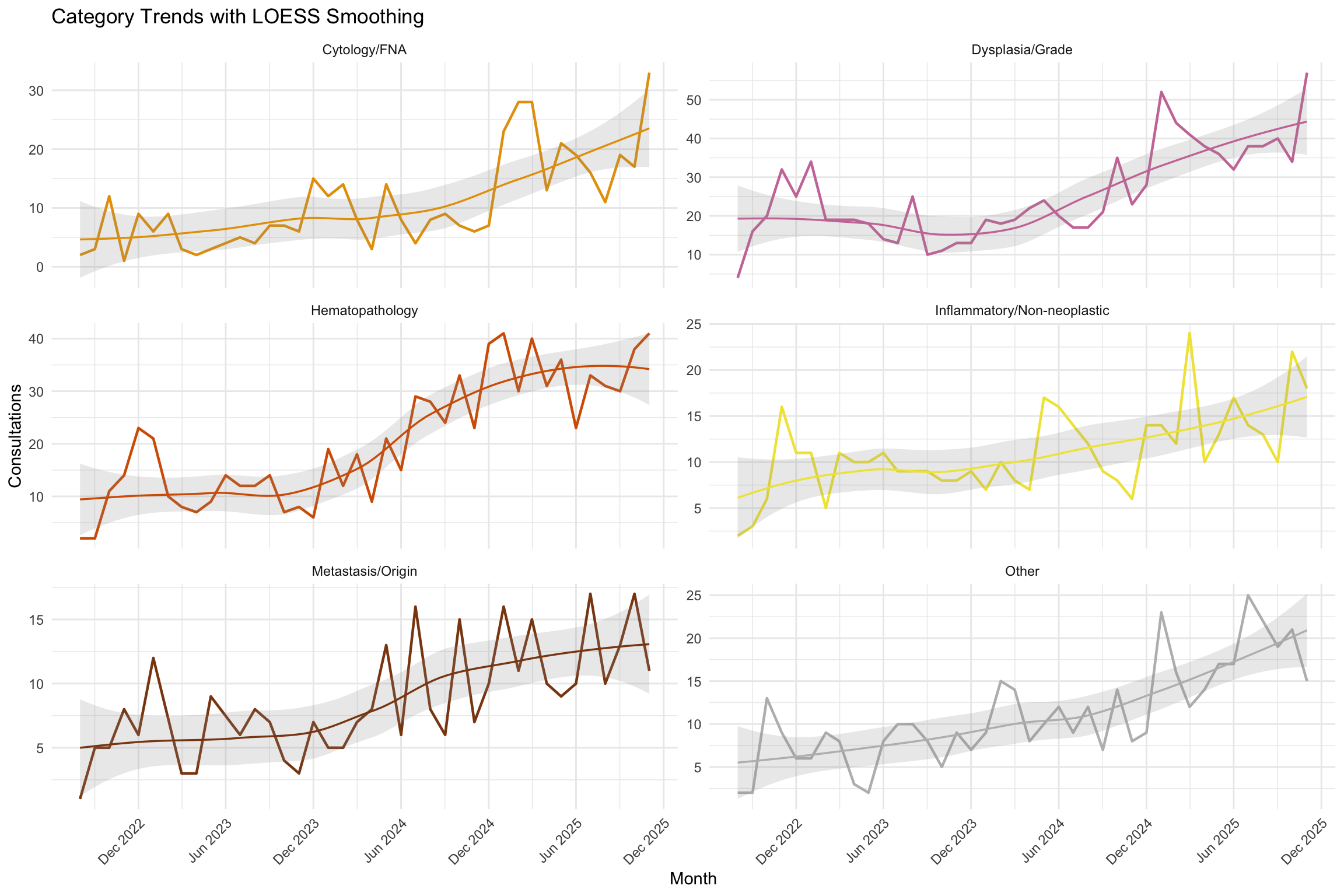
14.4 Category Trends Over Time
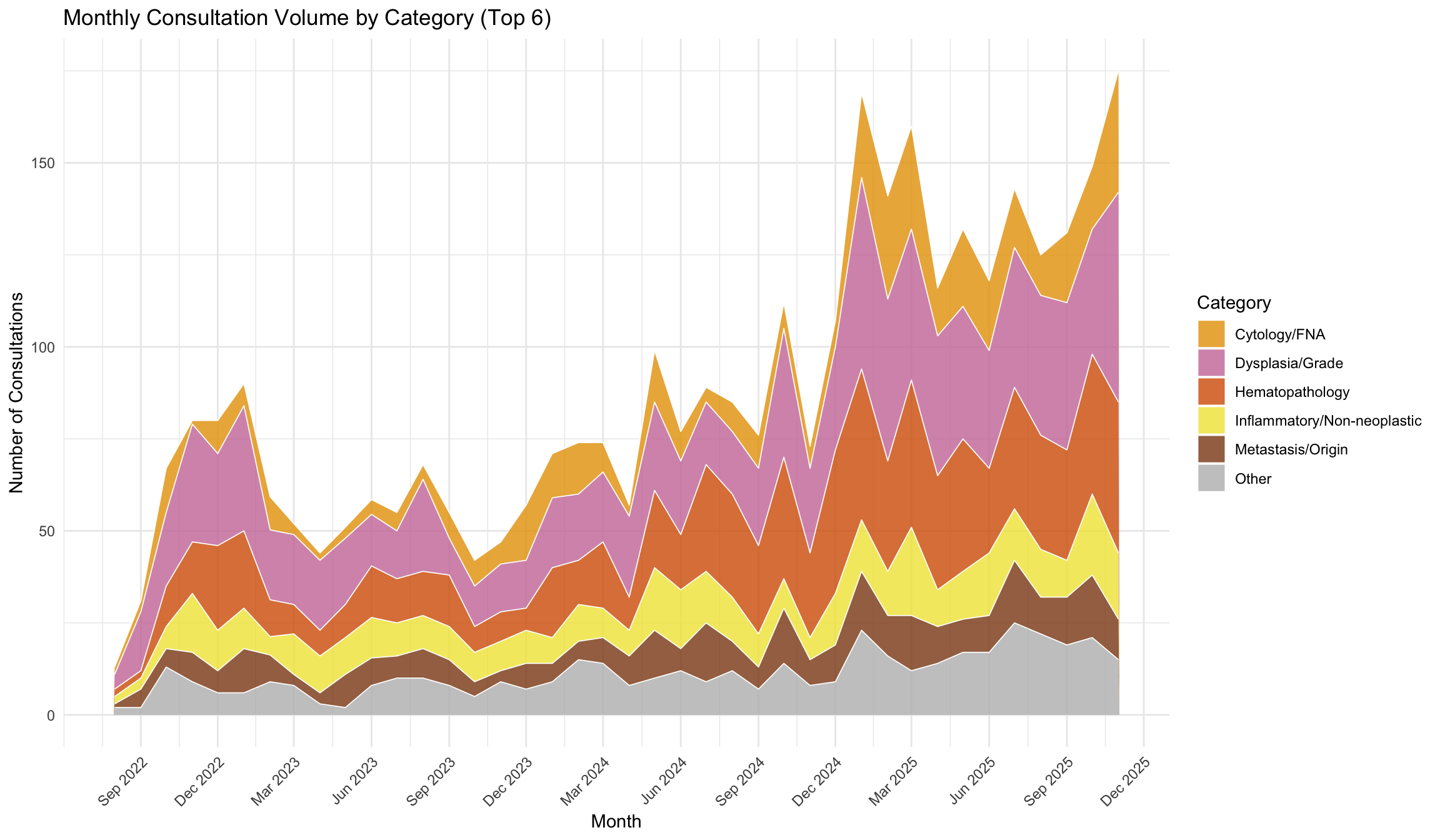
How have consultation topics evolved over time? This section tracks the monthly volume of the most common categories.
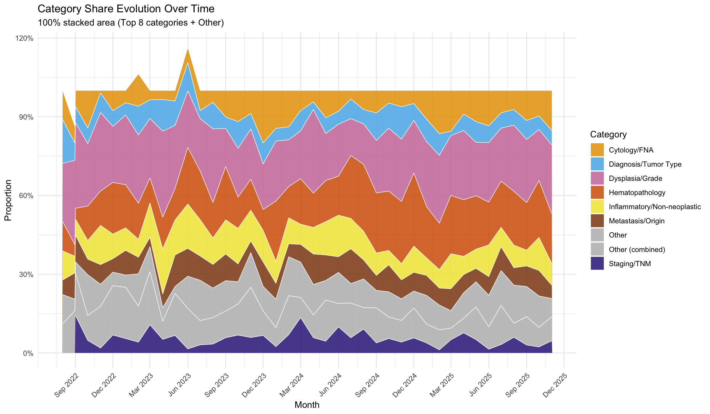
14.4.1 Category Share Evolution
Proportional representation of categories over time reveals shifts in consultation patterns.
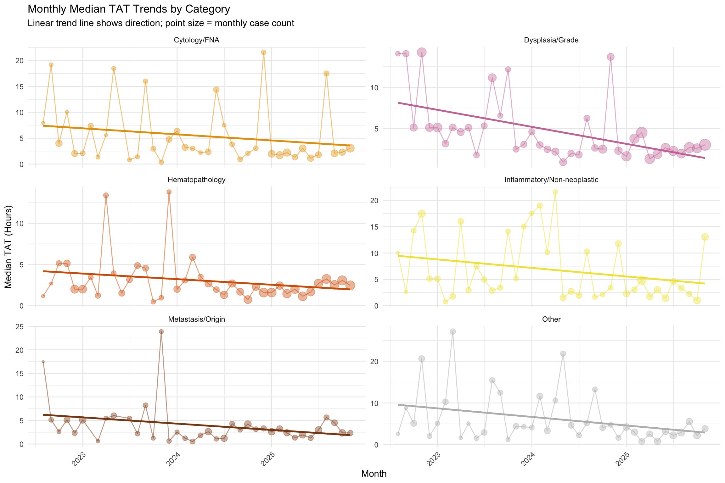
14.4.2 TAT Trends by Category
Are turnaround times improving or deteriorating for specific categories?
14.4.3 Emerging and Declining Topics
Which categories are growing or shrinking as a share of total consultations? Shifts in consultation topic distribution may reflect changes in case mix, evolving diagnostic criteria, or the impact of new technologies on pathology practice (Hanna et al. 2019; Bonert et al. 2021).
| Category | Total Cases | Avg Monthly % | Slope (logit/month) | P-Value | P-Adjusted (BH) | Direction |
|---|---|---|---|---|---|---|
| IHC/Biomarkers | 28 | 1.28 | -0.0294 | 0.0012 | 0.0052 | Decreasing |
| Neuroendocrine | 135 | 3.35 | -0.0251 | 0.0011 | 0.0052 | Decreasing |
| Second Opinion/Review | 52 | 1.74 | -0.0245 | 0.0191 | 0.0498 | Decreasing |
| Margin/Resection | 58 | 2.13 | -0.0229 | 0.0022 | 0.0072 | Decreasing |
| Hematopathology | 824 | 17.16 | 0.0209 | 0.0001 | 0.0012 | Increasing |
| Cytology/FNA | 422 | 9.09 | 0.0182 | 0.0345 | 0.0748 | Stable |
| Staging/TNM | 230 | 5.47 | -0.0125 | 0.1402 | 0.2025 | Stable |
| Sarcoma/Mesenchymal | 216 | 5.11 | -0.0121 | 0.0758 | 0.1231 | Stable |
| Inflammatory/Non-neoplastic | 443 | 10.32 | -0.0086 | 0.0661 | 0.1227 | Stable |
| Diagnosis/Tumor Type | 310 | 7.26 | -0.0083 | 0.1843 | 0.2178 | Stable |
| Other | 445 | 9.90 | 0.0078 | 0.1748 | 0.2178 | Stable |
| Dysplasia/Grade | 1018 | 22.62 | -0.0038 | 0.2944 | 0.3190 | Stable |
| Metastasis/Origin | 332 | 7.60 | 0.0015 | 0.7376 | 0.7376 | Stable |
14.5 Interrupted Time Series Analysis
The preceding trend analyses describe what happened over time. However, a simple trend line cannot tell us whether a specific event (such as a staffing change, new scanner deployment, or workflow reorganisation) caused a meaningful shift in consultation behaviour. Interrupted Time Series (ITS) analysis with segmented regression is considered one of the strongest quasi-experimental designs for evaluating pre/post intervention effects in observational data (Penfold and Zhang 2013; Bernal, Cummins, and Gasparrini 2017). It decomposes the time series into four components:
| Coefficient | Interpretation |
|---|---|
| B0 (intercept) | Baseline level at the start of the study |
| B1 (time) | Pre-intervention trend (slope per month) |
| B2 (intervention) | Immediate level change at the intervention point |
| B3 (time after) | Change in slope after the intervention |
NoteWhat does ITS add beyond simple trend analysis?
Simple linear or LOESS trends assume a single, smooth trajectory. ITS explicitly tests whether a particular time point marks a structural break — an abrupt shift in level (B2) and/or a change in the rate of change (B3). This separates observed differences from pre-existing trends and generally supports stronger quasi-experimental inference than a naive before/after comparison.
14.5.1 Data-Driven Changepoint Detection
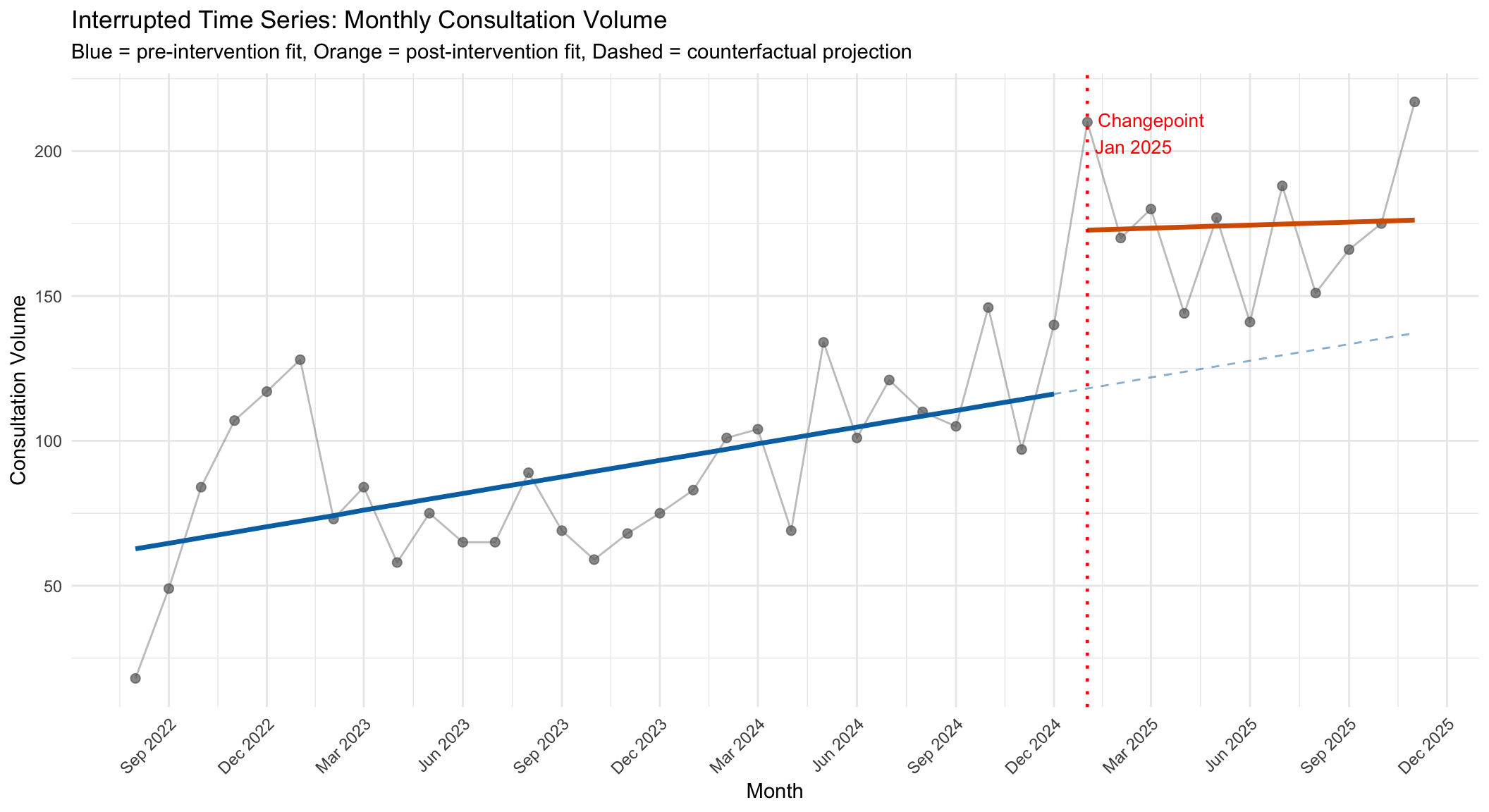
Because we do not have a single, externally defined intervention date, we adopt a data-driven strategy: we identify the month at which the largest absolute shift in the 3-month rolling average of consultation volume occurs, and treat that as the primary intervention point.
Detected changepoint: **January 2025** (month 30 of 40).
Pre-intervention: 29 months. Post-intervention: 11 months.
14.5.2 ITS Model: Consultation Volume
| Term | Estimate | Std. Error | 95% CI Lower | 95% CI Upper | P-value | |
|---|---|---|---|---|---|---|
| (Intercept) | Intercept (B0) | 60.815 | 9.635 | 41.274 | 80.356 | <0.001 |
| time | Pre-trend (B1) | 1.909 | 0.561 | 0.771 | 3.047 | 0.0016 |
| intervention | Level change (B2) | 54.646 | 17.208 | 19.747 | 89.544 | 0.0031 |
| time_after | Slope change (B3) | -1.563 | 2.474 | -6.582 | 3.455 | 0.5315 |
| Note: | ||||||
| P-values are conditional on the data-driven changepoint and are likely overstated (see warning below). |
WarningP-values are conditional on the data-driven changepoint
The changepoint was selected as the month with the largest absolute shift in the 3-month rolling average — i.e., the data were searched for the most extreme change. Consequently, the p-values for B2 (level change) are overstated because standard OLS inference does not account for this selection process. A formal structural break test (e.g., Andrews’ sup-F test) would provide valid p-values, but was not applied here. The B2 and B3 coefficients should be interpreted as descriptive effect estimates rather than formal hypothesis tests.
Interpretation. B1 captures the monthly trend in volume before the detected changepoint. B2 estimates the immediate jump (or drop) in volume at the changepoint. B3 indicates whether the monthly trend changed after the changepoint compared to the pre-intervention slope. A significant B2 suggests a sudden structural shift; a significant B3 suggests a sustained change in trajectory.
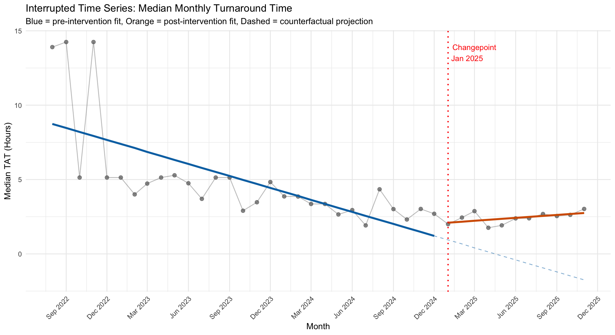
14.5.3 ITS Model: Median Turnaround Time
| Term | Estimate | Std. Error | 95% CI Lower | 95% CI Upper | P-value | |
|---|---|---|---|---|---|---|
| (Intercept) | Intercept (B0) | 9.006 | 0.810 | 7.363 | 10.648 | <0.001 |
| time | Pre-trend (B1) | -0.269 | 0.047 | -0.364 | -0.173 | <0.001 |
| intervention | Level change (B2) | 1.156 | 1.446 | -1.777 | 4.090 | 0.4292 |
| time_after | Slope change (B3) | 0.334 | 0.208 | -0.088 | 0.756 | 0.117 |
| Note: | ||||||
| P-values are conditional on the data-driven changepoint and are likely overstated (see warning above). |
14.5.4 ITS Residual Diagnostics
Before interpreting the ITS models, we verify key regression assumptions: normality and homoscedasticity of residuals.
| Diagnostic | Statistic | P-value / Magnitude | Interpretation |
|---|---|---|---|
| Residual normality: Volume (Shapiro-Wilk) | 0.9651 | 0.248 | Residuals approximately normal |
| Residual normality: TAT (Shapiro-Wilk) | 0.8420 | 5.8e-05 | Non-normal residuals (interpret CIs with caution) |
| Heteroscedasticity: Volume (Breusch-Pagan) | 4.0500 | 0.256 | No heteroscedasticity |
| Heteroscedasticity: TAT (Breusch-Pagan) | 17.1420 | 0.000661 | Heteroscedasticity present |
| Intervention effect size: Volume (Cohen's f2) | 0.3377 | medium | R2 change from adding intervention terms: 8.8pp |
| Intervention effect size: TAT (Cohen's f2) | 0.1931 | medium | R2 change from adding intervention terms: 8.7pp |
NoteCohen’s f2 for ITS
Cohen’s f2 quantifies the incremental explanatory power of the intervention terms (level change B2 and slope change B3) beyond the baseline time trend (B1). Benchmarks: f2 < 0.02 negligible, 0.02–0.15 small, 0.15–0.35 medium, > 0.35 large (Cohen, 1988).
14.5.5 Autocorrelation Diagnostics
A key assumption of ordinary least squares regression is that residuals are independent. Time series data often violate this assumption because consecutive months tend to be correlated (autocorrelation). The Durbin-Watson test formally checks for first-order autocorrelation in the residuals.
| Outcome | DW Statistic | P-value | Interpretation |
|---|---|---|---|
| Consultation Volume | 1.418 | 0.0080 | Significant autocorrelation detected |
| Median TAT | 1.686 | 0.0656 | No significant autocorrelation |
Autocorrelation detected in at least one model. Refitting with generalised least squares (GLS) using an AR(1) correlation structure to obtain corrected standard errors.
| Term | Estimate | Std. Error | P-value | |
|---|---|---|---|---|
| (Intercept) | Intercept (B0) | 57.309 | 15.067 | <0.001 |
| time | Pre-trend (B1) | 2.043 | 0.863 | 0.0234 |
| intervention | Level change (B2) | 55.498 | 22.567 | 0.0189 |
| time_after | Slope change (B3) | -1.264 | 3.489 | 0.7191 |
Estimated AR(1) autocorrelation coefficient (phi): 0.409
14.5.6 ITS Model Summary
| Metric | Consultation Volume | Median TAT (Hours) |
|---|---|---|
| R-squared | 0.739 | 0.551 |
| Adjusted R-squared | 0.717 | 0.513 |
| Mean (Pre) | 89.4 | 5 |
| Mean (Post) | 174.5 | 2.4 |
| Change (%) | +95% | -51.3% |
The ITS analysis provides a rigorous framework for assessing whether the observed changes around January 2025 represent a genuine structural break or are merely a continuation of pre-existing trends. Unlike simple before/after comparisons, which confound the intervention effect with underlying temporal dynamics, the segmented regression model explicitly separates the pre-existing trend (B1) from the immediate level shift (B2) and the post-intervention trend change (B3). This decomposition strengthens the basis for causal inference, though — as with all observational designs — unmeasured confounders (such as concurrent staffing changes or case-mix shifts) cannot be entirely ruled out (Penfold and Zhang 2013).
WarningLimitations of Data-Driven Changepoint Selection
The changepoint was selected by the data itself (the month with the largest shift in rolling average), rather than being specified a priori based on a known intervention. This approach is exploratory rather than confirmatory: the statistical significance of B2 and B3 may be inflated because the changepoint was chosen to maximise the observed shift. The ITS results should therefore be interpreted as hypothesis-generating rather than hypothesis-confirming. If a specific known intervention date exists (e.g., scanner deployment, staffing change), the analysis should be re-run with that date fixed a priori to obtain valid inferential statistics.