[1] TRUE8 Statistical Analysis
This chapter presents comprehensive statistical tests to examine relationships and patterns in the consultation data. Non-parametric methods are used throughout given the typically right-skewed distribution of turnaround times in pathology practice (Volmar et al. 2015; Sharma et al. 2025). Where multiple comparisons are performed, Benjamini-Hochberg correction is applied to control the false discovery rate.
8.1 Consultation Volume and Turnaround Time Correlation
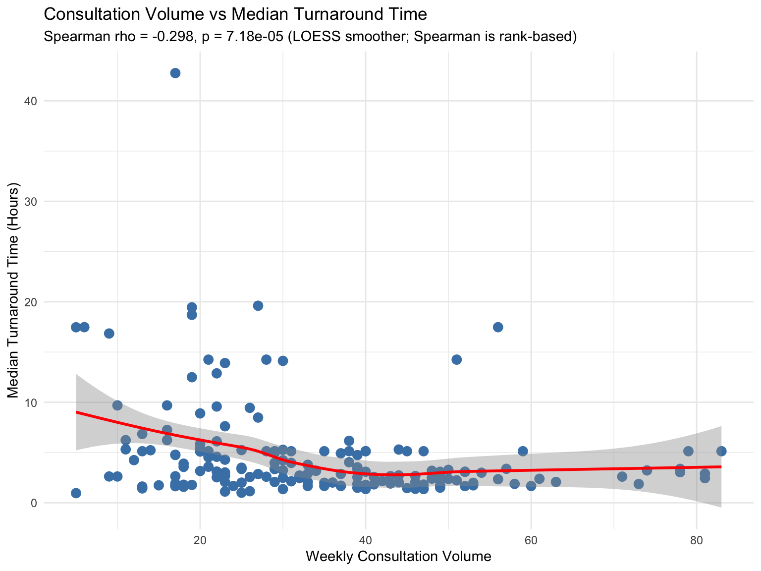
Research Question: Is there a relationship between consultation volume and turnaround times? Turnaround time is a key quality metric in surgical pathology, with institutional benchmarks typically set at 24–48 hours for routine cases (Volmar et al. 2015; Sharma et al. 2025; Ardon et al. 2023).
8.1.1 Volume vs TAT by Month
| Month | Volume | Median_TAT | Mean_TAT | SD_TAT |
|---|---|---|---|---|
| 2022-08 | 27 | 13.91 | 11.20 | 7.84 |
| 2022-09 | 59 | 14.25 | 13.04 | 14.61 |
| 2022-10 | 124 | 5.14 | 9.46 | 9.94 |
| 2022-11 | 192 | 14.25 | 13.03 | 13.41 |
| 2022-12 | 197 | 5.14 | 8.45 | 9.41 |
| 2023-01 | 208 | 5.14 | 10.34 | 14.71 |
| 2023-02 | 96 | 4.00 | 13.81 | 21.17 |
| 2023-03 | 119 | 4.73 | 16.41 | 23.48 |
| 2023-04 | 77 | 5.14 | 17.02 | 23.44 |
| 2023-05 | 96 | 5.29 | 14.36 | 21.33 |
| 2023-06 | 77 | 4.75 | 15.79 | 23.39 |
| 2023-07 | 87 | 3.70 | 12.81 | 20.67 |
| 2023-08 | 119 | 5.14 | 14.75 | 19.64 |
| 2023-09 | 90 | 5.14 | 16.38 | 24.01 |
| 2023-10 | 66 | 2.90 | 14.77 | 22.72 |
| 2023-11 | 85 | 3.47 | 17.10 | 24.42 |
| 2023-12 | 86 | 4.83 | 13.07 | 18.33 |
| 2024-01 | 90 | 3.87 | 11.24 | 15.64 |
| 2024-02 | 123 | 3.86 | 14.84 | 21.67 |
| 2024-03 | 124 | 3.36 | 8.16 | 12.61 |
| 2024-04 | 79 | 3.36 | 13.35 | 21.21 |
| 2024-05 | 159 | 2.65 | 9.48 | 15.21 |
| 2024-06 | 124 | 2.95 | 10.97 | 16.11 |
| 2024-07 | 142 | 1.92 | 8.06 | 14.48 |
| 2024-08 | 118 | 4.34 | 12.54 | 16.63 |
| 2024-09 | 112 | 3.01 | 9.69 | 15.50 |
| 2024-10 | 169 | 2.31 | 9.58 | 15.44 |
| 2024-11 | 117 | 3.02 | 10.18 | 14.83 |
| 2024-12 | 161 | 2.70 | 10.17 | 15.97 |
| 2025-01 | 241 | 2.00 | 8.13 | 13.86 |
| 2025-02 | 203 | 2.44 | 7.40 | 11.58 |
| 2025-03 | 261 | 2.88 | 9.94 | 15.31 |
| 2025-04 | 199 | 1.76 | 7.80 | 13.26 |
| 2025-05 | 240 | 1.92 | 6.00 | 10.93 |
| 2025-06 | 195 | 2.39 | 7.44 | 12.82 |
| 2025-07 | 228 | 2.39 | 8.38 | 15.29 |
| 2025-08 | 192 | 2.68 | 7.86 | 12.57 |
| 2025-09 | 231 | 2.55 | 10.03 | 16.83 |
| 2025-10 | 234 | 2.62 | 8.99 | 14.21 |
| 2025-11 | 288 | 3.02 | 8.43 | 13.05 |
| 2025-12 | 47 | 1.80 | 5.31 | 8.52 |
Spearman Correlation Test:
| Metric | Value |
|---|---|
| Correlation Coefficient (rho) | -0.298 |
| 95% CI (bootstrap) | [-0.436, -0.141] |
| P-value | 7.18e-05 |
| Interpretation | Statistically significant |
8.2 Day of Week Effects
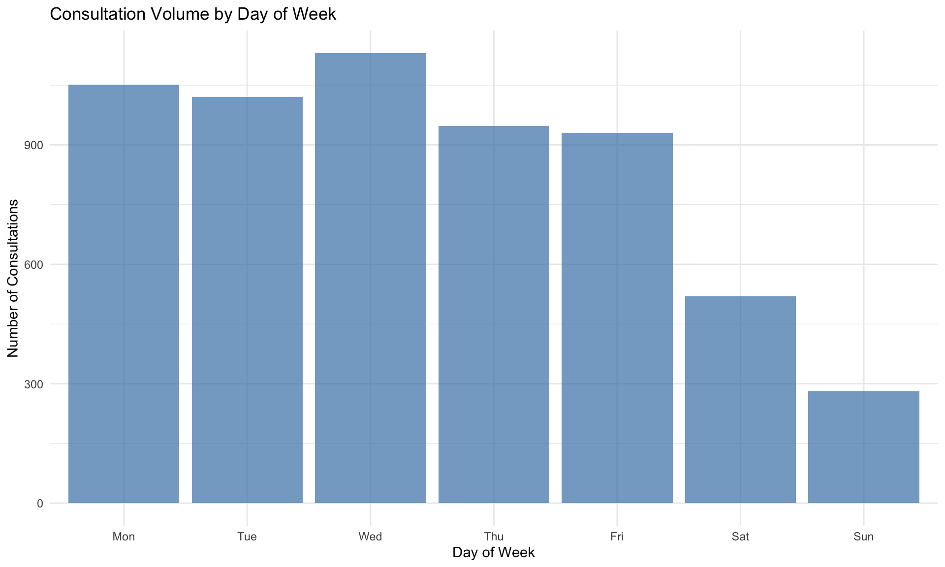
Research Question: Does the day of the week affect consultation patterns or turnaround times? Temporal variation in consultation volume has been observed in studies of intradepartmental consultation workflows (Goebel, Ettler, and Walsh 2018; Dunbar et al. 2022).
8.2.1 Consultation Volume by Day of Week
| DayOfWeek | Count | Median_TAT | Mean_TAT | SD_TAT | Q1 | Q3 |
|---|---|---|---|---|---|---|
| Mon | 1051 | 2.67 | 8.79 | 13.90 | 0.88 | 13.62 |
| Tue | 1021 | 2.62 | 8.01 | 12.45 | 0.96 | 11.52 |
| Wed | 1131 | 2.76 | 8.00 | 11.86 | 0.89 | 12.63 |
| Thu | 948 | 2.62 | 9.16 | 15.50 | 0.81 | 14.16 |
| Fri | 930 | 3.02 | 11.58 | 19.86 | 0.89 | 14.25 |
| Sat | 520 | 4.45 | 17.77 | 22.16 | 1.66 | 36.65 |
| Sun | 281 | 16.18 | 19.32 | 17.72 | 10.34 | 20.42 |
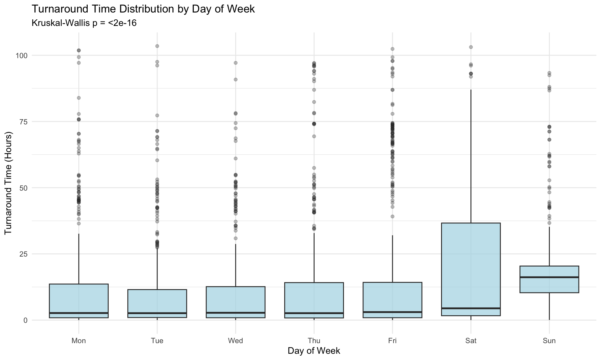
8.2.2 Kruskal-Wallis Test: TAT by Day of Week
Non-parametric test to compare turnaround times across days of the week:
| Metric | Value |
|---|---|
| Chi-squared statistic | 251.374 |
| Degrees of freedom | 6 |
| P-value | <2e-16 |
| Effect size (epsilon-squared) | 0.0418 |
| Interpretation | Significant, small effect |
| Comparison | Z | P.unadj | P.adj |
|---|---|---|---|
| Sun - Wed | 13.2021 | 0 | 0 |
| Mon - Sun | -13.0978 | 0 | 0 |
| Sun - Tue | 13.1180 | 0 | 0 |
| Sun - Thu | 12.9375 | 0 | 0 |
| Fri - Sun | -12.0508 | 0 | 0 |
| Sat - Wed | 7.0191 | 0 | 0 |
| Sat - Tue | 6.9720 | 0 | 0 |
| Mon - Sat | -6.9296 | 0 | 0 |
| Sat - Sun | -6.8625 | 0 | 0 |
| Sat - Thu | 6.7924 | 0 | 0 |
8.3 Hour of Day Effects
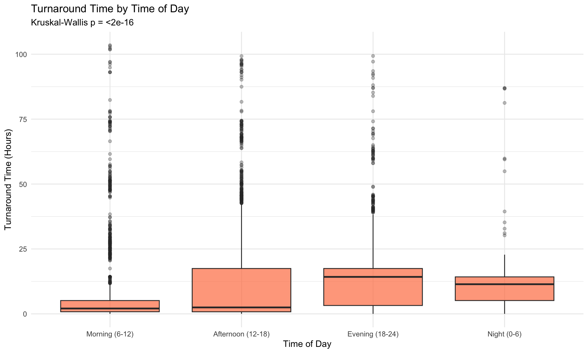
Research Question: Does the time of day when a consultation is initiated affect turnaround time?
| TimeOfDay | Count | Median_TAT | Mean_TAT | SD_TAT |
|---|---|---|---|---|
| Morning (6-12) | 2042 | 2.07 | 7.34 | 14.84 |
| Afternoon (12-18) | 2692 | 2.49 | 10.27 | 16.60 |
| Evening (18-24) | 945 | 14.25 | 16.20 | 16.11 |
| Night (0-6) | 203 | 11.42 | 13.04 | 13.49 |
8.3.1 Kruskal-Wallis Test: TAT by Time of Day
| Metric | Value |
|---|---|
| Chi-squared statistic | 460.427 |
| Degrees of freedom | 3 |
| P-value | <2e-16 |
| Effect size (epsilon-squared) | 0.0778 |
| Interpretation | Significant, moderate effect |
| Comparison | Z | P.unadj | P.adj |
|---|---|---|---|
| Afternoon (12-18) - Evening (18-24) | -16.0832 | 0.0000 | 0.0000 |
| Afternoon (12-18) - Morning (6-12) | 5.1769 | 0.0000 | 0.0000 |
| Evening (18-24) - Morning (6-12) | 19.3181 | 0.0000 | 0.0000 |
| Afternoon (12-18) - Night (0-6) | -9.2032 | 0.0000 | 0.0000 |
| Evening (18-24) - Night (0-6) | -0.7980 | 0.4249 | 0.4249 |
| Morning (6-12) - Night (0-6) | -11.1665 | 0.0000 | 0.0000 |
8.4 Comparison of TAT Across Responders
Research Question: Do different responders have significantly different turnaround times? Inter-pathologist variability in consultation response patterns has implications for quality assurance and workload distribution (Renshaw et al. 2002; Nakhleh et al. 2016; Bonert et al. 2022).
| Metric | Value |
|---|---|
| Chi-squared statistic | 711.028 |
| Degrees of freedom | 22 |
| P-value | <2e-16 |
| Effect size (epsilon-squared) | 0.1183 |
| Interpretation | Significant, moderate effect |
| Comparison | Z | P.unadj | P.adj |
|---|---|---|---|
| P11 - P17 | -16.5073 | 0 | 0 |
| P17 - P5 | 15.3157 | 0 | 0 |
| P17 - P2 | 15.1892 | 0 | 0 |
| P11 - P33 | -13.8772 | 0 | 0 |
| P10 - P17 | -13.1448 | 0 | 0 |
| P33 - P5 | 12.5664 | 0 | 0 |
| P2 - P33 | -12.5105 | 0 | 0 |
| P17 - P24 | 12.4414 | 0 | 0 |
| P17 - P27 | 11.6701 | 0 | 0 |
| P10 - P33 | -11.4491 | 0 | 0 |
8.4.1 Responder TAT Summary
| Responder | N | Median_TAT | Mean_TAT | SD_TAT |
|---|---|---|---|---|
| P27 | 94 | 1.13 | 4.68 | 9.53 |
| P24 | 120 | 1.30 | 5.07 | 11.68 |
| P10 | 216 | 1.36 | 6.76 | 12.92 |
| P11 | 522 | 1.67 | 5.37 | 9.65 |
| P13 | 68 | 1.78 | 7.32 | 13.47 |
| P5 | 751 | 1.99 | 7.58 | 14.02 |
| P2 | 684 | 2.07 | 6.53 | 12.59 |
| P19 | 227 | 2.62 | 7.86 | 12.95 |
| P23 | 407 | 3.02 | 7.11 | 10.35 |
| P28 | 124 | 3.05 | 9.81 | 16.03 |
| P8 | 348 | 3.36 | 11.73 | 19.59 |
| P30 | 18 | 3.44 | 6.94 | 8.13 |
| P21 | 399 | 3.70 | 12.29 | 16.65 |
| P18 | 83 | 4.01 | 8.51 | 13.35 |
| P9 | 696 | 5.14 | 10.09 | 14.21 |
| P3 | 15 | 5.49 | 13.22 | 17.78 |
| P25 | 17 | 6.07 | 11.22 | 12.49 |
| P4 | 79 | 8.86 | 12.10 | 14.53 |
| P1 | 29 | 13.91 | 14.97 | 18.27 |
| P6 | 254 | 14.25 | 17.93 | 21.49 |
| P33 | 261 | 17.48 | 19.16 | 18.04 |
| P16 | 75 | 18.10 | 18.50 | 18.39 |
| P17 | 362 | 20.29 | 24.46 | 23.86 |
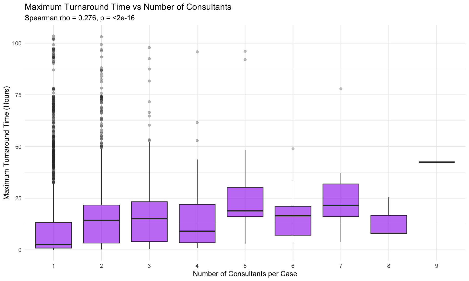
8.5 Number of Consultants vs TAT
Research Question: Does involving more consultants lead to longer total response times? Cases requiring multiple opinions are often diagnostically complex and may reflect the inherent difficulty documented in second-opinion pathology studies (Peck et al. 2018; Elmore et al. 2015; Farooq et al. 2021).
| Metric | Value |
|---|---|
| Correlation Coefficient (rho) | 0.276 |
| 95% CI (bootstrap) | [0.251, 0.3] |
| P-value | <2e-16 |
| Effect size magnitude | small |
| Interpretation | Statistically significant, small effect |
8.6 Temporal Trend Analysis
Research Question: Is there a statistically significant trend in consultation volumes over time? Increasing adoption of digital pathology platforms has been associated with changes in consultation volume and practice patterns over time (Hanna et al. 2019, 2022).
8.6.1 Adjusted Mann-Kendall Trend Test
| Metric | Value |
|---|---|
| Method | TFPW Mann-Kendall (monthly deseasonalized) |
| Tau statistic | 0.492 |
| P-value (two-tailed) | 8.11e-06 |
| Lag-1 rho | 0.474 |
| Interpretation | Significant increasing trend |
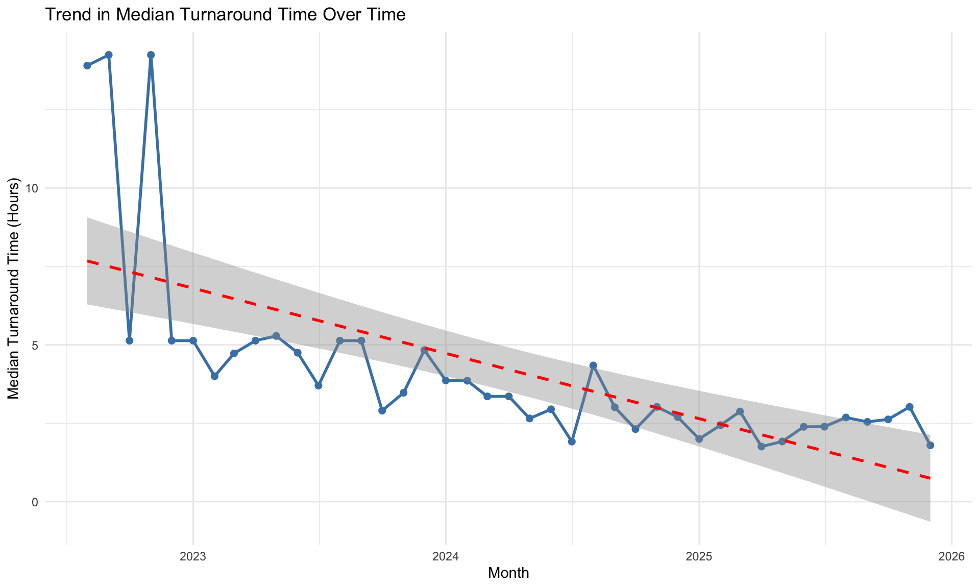
8.6.2 Trend in Median TAT Over Time
| Metric | Value |
|---|---|
| Method | TFPW Mann-Kendall (monthly deseasonalized) |
| Tau statistic | -0.562 |
| P-value (two-tailed) | 3.55e-07 |
| Lag-1 rho | 0.251 |
| Interpretation | Significant decreasing trend |
8.7 Multiple Regression Analysis
Research Question: What factors predict turnaround time? Identifying predictors of consultation TAT is important for quality management and operational planning in pathology departments (Ardon et al. 2023; Bonert et al. 2021).
8.7.1 Predicting TAT from Multiple Factors
| term | estimate | std.error | statistic | p.value |
|---|---|---|---|---|
| (Intercept) | 0.889 | 0.067 | 13.223 | 0.000 |
| IsWeekend | 0.639 | 0.043 | 14.740 | 0.000 |
| Hour | 0.049 | 0.003 | 14.364 | 0.000 |
| Month_Num2 | -0.022 | 0.074 | -0.292 | 0.770 |
| Month_Num3 | -0.078 | 0.071 | -1.107 | 0.268 |
| Month_Num4 | -0.058 | 0.078 | -0.748 | 0.455 |
| Month_Num5 | -0.154 | 0.071 | -2.183 | 0.029 |
| Month_Num6 | -0.092 | 0.075 | -1.229 | 0.219 |
| Month_Num7 | -0.152 | 0.072 | -2.100 | 0.036 |
| Month_Num8 | 0.038 | 0.072 | 0.527 | 0.598 |
| Month_Num9 | 0.094 | 0.071 | 1.333 | 0.183 |
| Month_Num10 | 0.013 | 0.068 | 0.198 | 0.843 |
| Month_Num11 | 0.126 | 0.065 | 1.917 | 0.055 |
| Month_Num12 | 0.087 | 0.071 | 1.227 | 0.220 |
| Case_Complexity | 0.043 | 0.012 | 3.568 | 0.000 |
8.7.2 Model Summary Statistics
| Metric | Value |
|---|---|
| R-squared | 0.0813 |
| Adjusted R-squared | 0.0791 |
| F-statistic | 37.1 |
| P-value | <2e-16 |
| AIC | 18191.93 |
8.7.3 Regression Assumption Diagnostics
| Diagnostic Test | Statistic | P-value | Interpretation |
|---|---|---|---|
| Shapiro-Wilk normality of residuals (tested on random subsample of 5,000 from 5,882 residuals) | 0.9672 | <2e-16 | Residuals deviate from normality (expected with large N; OLS estimates remain consistent via CLT) |
| Breusch-Pagan heteroscedasticity | 61.8680 | 5.5e-08 | Heteroscedasticity detected (consider robust SEs or WLS) |
| VIF (max value) | 11.0000 | 11 (concern) | Possible multicollinearity |
Model Interpretation:
The model is fit on log(TAT+1), so coefficients represent multiplicative effects. To interpret a coefficient b: exp(b) gives the multiplicative change in (TAT+1) for a one-unit increase in the predictor.
- IsWeekend: Consultations initiated on weekends may have longer TAT if staff availability is reduced, or shorter TAT if weekend cases are pre-screened.
- Hour: Earlier or later hours of the day may systematically affect response speed due to staffing patterns.
- Month_Num (factor): Captures seasonal effects — e.g., summer months may show different TAT due to vacation coverage. Treated as a categorical variable to allow non-linear seasonal patterns.
- Case_Complexity: Cases requiring multiple consultants tend to be diagnostically complex and may take longer.
Significant predictors (p < 0.05) have a statistically significant association with turnaround time, though the model explains only a modest fraction of TAT variance, suggesting that individual case-level factors dominate.
8.8 Mixed Effects Models: Accounting for Pathologist-Level Clustering
Standard statistical tests (Kruskal-Wallis, Spearman, OLS regression) assume that observations are independent. In consultation data, however, this assumption is violated: multiple consultations answered by the same pathologist are correlated because each pathologist brings a characteristic response style, subspecialty expertise, and workload capacity. Ignoring this clustering inflates Type I error rates and produces overconfident standard errors (Nakhleh et al. 2016; Bonert et al. 2022).
Mixed effects models (also called multilevel or hierarchical models) address this by partitioning variance into fixed effects (population-level predictors like weekend or time of day) and random effects (pathologist-specific deviations). The random intercept for each responder captures that pathologist’s baseline tendency to respond faster or slower than average, after accounting for fixed effects.
NoteWhy Mixed Effects Models?
In this dataset, each responder contributes dozens to hundreds of consultations. A standard regression treats each consultation as fully independent, but consultations handled by the same pathologist share a common “baseline speed.” Mixed effects models explicitly model this structure, yielding:
- Correct standard errors that account for within-pathologist correlation
- Intraclass Correlation Coefficient (ICC): the proportion of total variance attributable to between-pathologist differences
- Pathologist-specific estimates (random effects) showing who is systematically faster or slower, with proper uncertainty quantification
8.8.1 Model 1: Random Intercept Only (Null Model)
The simplest mixed model includes only a random intercept for each responder, with no fixed-effect predictors. This partitions the total variance in log(TAT) into between-pathologist and within-pathologist components.
| Component | Value |
|---|---|
| Between-pathologist variance (tau^2) | 0.4381 |
| Within-pathologist variance (sigma^2) | 2.7487 |
| Total variance | 3.1869 |
| ICC (Intraclass Correlation) | 13.7% |
TipInterpreting the ICC
The ICC indicates the proportion of total TAT variability explained by who the responder is. An ICC of 10–20% is common in healthcare quality studies and indicates that pathologist identity meaningfully influences response time, even after accounting for case-level factors. An ICC near zero would suggest that individual pathologist differences are negligible relative to case-to-case variation. Values above 20% indicate strong pathologist-level clustering, reinforcing the need for hierarchical modelling.
8.8.2 Model 2: Full Model with Fixed Effects
This model adds fixed-effect predictors for factors that may influence turnaround time:
- Weekend (Weekday vs Weekend): reduced staffing on weekends may delay responses
- Hour_Category: time-of-day when consultation was initiated
- Question_Category: the topic or type of consultation question
| Term | Estimate | Std. Error | df | t value | Pr(>|t|) | Significance | Exp(Estimate) | |
|---|---|---|---|---|---|---|---|---|
| (Intercept) | (Intercept) | 0.890 | 0.150 | 41.203 | 5.922 | 0.000 | *** | 2.435 |
| WeekendWeekend | WeekendWeekend | 0.714 | 0.061 | 5812.476 | 11.690 | 0.000 | *** | 2.041 |
| Hour_CategoryAfternoon (12-18) | Hour_CategoryAfternoon (12-18) | 0.224 | 0.047 | 5814.047 | 4.765 | 0.000 | *** | 1.252 |
| Hour_CategoryEvening (18-24) | Hour_CategoryEvening (18-24) | 1.105 | 0.065 | 5825.132 | 17.025 | 0.000 | *** | 3.020 |
| Hour_CategoryNight (0-6) | Hour_CategoryNight (0-6) | 1.029 | 0.122 | 5831.806 | 8.454 | 0.000 | *** | 2.798 |
| Question_CategoryDiagnosis/Tumor Type | Question_CategoryDiagnosis/Tumor Type | -0.160 | 0.110 | 5820.497 | -1.454 | 0.146 | 0.852 | |
| Question_CategoryDysplasia/Grade | Question_CategoryDysplasia/Grade | -0.093 | 0.088 | 5827.629 | -1.050 | 0.294 | 0.911 | |
| Question_CategoryHematopathology | Question_CategoryHematopathology | -0.336 | 0.090 | 5826.497 | -3.739 | 0.000 | *** | 0.714 |
| Question_CategoryIHC/Biomarkers | Question_CategoryIHC/Biomarkers | 0.326 | 0.268 | 5813.300 | 1.216 | 0.224 | 1.386 | |
| Question_CategoryInflammatory/Non-neoplastic | Question_CategoryInflammatory/Non-neoplastic | -0.172 | 0.100 | 5820.863 | -1.717 | 0.086 | . | 0.842 |
| Question_CategoryMargin/Resection | Question_CategoryMargin/Resection | 0.128 | 0.199 | 5817.012 | 0.644 | 0.520 | 1.136 | |
| Question_CategoryMetastasis/Origin | Question_CategoryMetastasis/Origin | -0.213 | 0.107 | 5829.430 | -1.985 | 0.047 | * | 0.808 |
| Question_CategoryNeuroendocrine | Question_CategoryNeuroendocrine | -0.042 | 0.138 | 5817.966 | -0.303 | 0.762 | 0.959 | |
| Question_CategoryOther | Question_CategoryOther | -0.107 | 0.101 | 5818.790 | -1.059 | 0.290 | 0.899 | |
| Question_CategorySarcoma/Mesenchymal | Question_CategorySarcoma/Mesenchymal | -0.143 | 0.119 | 5820.204 | -1.205 | 0.228 | 0.866 | |
| Question_CategorySecond Opinion/Review | Question_CategorySecond Opinion/Review | -0.231 | 0.207 | 5817.421 | -1.118 | 0.264 | 0.793 | |
| Question_CategoryStaging/TNM | Question_CategoryStaging/TNM | 0.004 | 0.119 | 5823.716 | 0.034 | 0.973 | 1.004 | |
| Note: | ||||||||
| Exp(Estimate) represents the multiplicative change in TAT. Values > 1 indicate longer TAT; < 1 indicate shorter TAT. Significance: *** p<0.001, ** p<0.01, * p<0.05, . p<0.10 |
| Component | Value |
|---|---|
| Between-pathologist variance (tau^2) | 0.3494 |
| Within-pathologist variance (sigma^2) | 2.5209 |
| Conditional ICC | 12.2% |
| Residual variance reduction vs null model | 8.3% |
8.8.3 Mixed Model Diagnostics
| Diagnostic | Value | Interpretation |
|---|---|---|
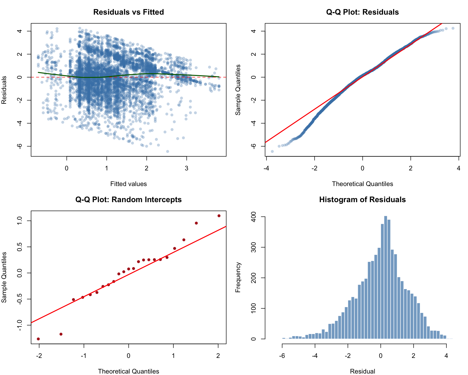
| Residual normality (Shapiro-Wilk) (subsample of 5,000 from 5,849) | W = 0.9875, p = <2e-16 | Residuals deviate from normality (common with large N; inference robust via asymptotic theory) |
| Random intercept normality (Shapiro-Wilk) | W = 0.9593, p = 0.449 | Random intercepts approximately normal |
| Residual SD | 1.5828 | |
| Random intercept SD | 0.5661 |
Diagnostic plots for the full mixed effects model. Top-left: residuals vs fitted values (checking homoscedasticity). Top-right: Q-Q plot of residuals (checking normality). Bottom-left: Q-Q plot of random effects (checking normality of random intercepts). Bottom-right: histogram of residuals.
8.8.4 Model Comparison
Comparing models using AIC and BIC helps assess whether the added fixed effects meaningfully improve fit. Lower values indicate better fit, with BIC imposing a stronger penalty for model complexity.
| Model | AIC | BIC | logLik |
|---|---|---|---|
| OLS (no random effects) | 23180.8 | 23194.2 | -11588.4 |
| Mixed: Random intercept only | 22592.3 | 22612.3 | -11293.2 |
| Mixed: Full model (fixed + random) | 22099.2 | 22226.0 | -11030.6 |
| Comparison | Chi-sq | P-value | Interpretation |
|---|---|---|---|
| Null mixed model vs Full mixed model | 525.117 | <2e-16 | Fixed effects significantly improve model fit |
8.8.5 Caterpillar Plot: Pathologist Random Effects
The caterpillar plot displays each responder’s estimated random intercept (deviation from the population mean) with 95% conditional intervals. Intervals fully above or below zero indicate stronger model-based evidence of slower or faster baseline response tendency, respectively. These are shrinkage-based uncertainty intervals for random effects, not standalone per-pathologist hypothesis tests (Bonert et al. 2022).
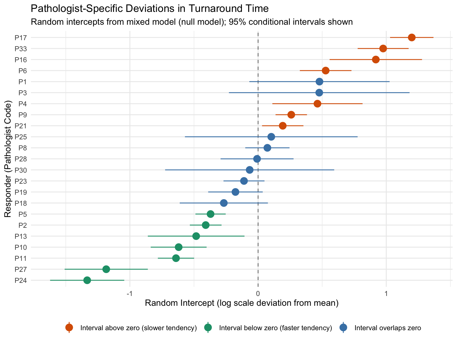
Among 23 pathologists with >= 10 consultations, 7 have conditional intervals entirely below zero (faster tendency) and 7 have intervals entirely above zero (slower tendency). The fastest pathologist’s baseline TAT is approximately 0.26x the population geometric mean, while the slowest is approximately 3.32x the population geometric mean.
8.8.6 Mixed Effects Summary
| Metric | Value |
|---|---|
| Observations (N) | 5,849 |
| Number of responders | 23 |
| ICC (null model) | 13.7% |
| AIC improvement (null mixed vs OLS) | 588.5 units |
| Pathologists with interval below zero | 7 |
| Pathologists with interval above zero | 7 |
| Full model LRT p-value | <2e-16 |
8.9 Summary of Statistical Findings
This chapter applied eight analytical approaches across multiple research questions, including hierarchical modelling via mixed effects to account for pathologist-level clustering. All post-hoc pairwise comparisons (Dunn tests) used Benjamini-Hochberg correction to control the false discovery rate within each family of comparisons. While the three primary Kruskal-Wallis tests (day of week, time of day, responder) address distinct research questions and thus were not further adjusted across families, readers should interpret borderline significant results (0.01 < p < 0.05) with appropriate caution given the overall number of tests performed.
| Research Question | Statistical Test | Effect Size | P-value | Result |
|---|---|---|---|---|
| Volume vs TAT correlation | Spearman correlation | rho = -0.298 | 7.18e-05 | Significant |
| Day of week effect on TAT | Kruskal-Wallis | eps2 = 0.0418 (small) | <2e-16 | Significant |
| Time of day effect on TAT | Kruskal-Wallis | eps2 = 0.0778 (moderate) | <2e-16 | Significant |
| Responder differences | Kruskal-Wallis | eps2 = 0.1183 (moderate) | <2e-16 | Significant |
| Number of consultants vs TAT | Spearman correlation | rho = 0.276 | <2e-16 | Significant |
| Temporal trend in volume | Adjusted Mann-Kendall | tau = 0.492 | 8.11e-06 | Significant trend |
| Temporal trend in TAT | Adjusted Mann-Kendall | tau = -0.562 | 3.55e-07 | Significant trend |
| Pathologist-level clustering (ICC) | Mixed effects (lmer) | ICC = 13.7% | <2e-16 | ICC = 13.7% |