17  Predictive Models and Forecasting

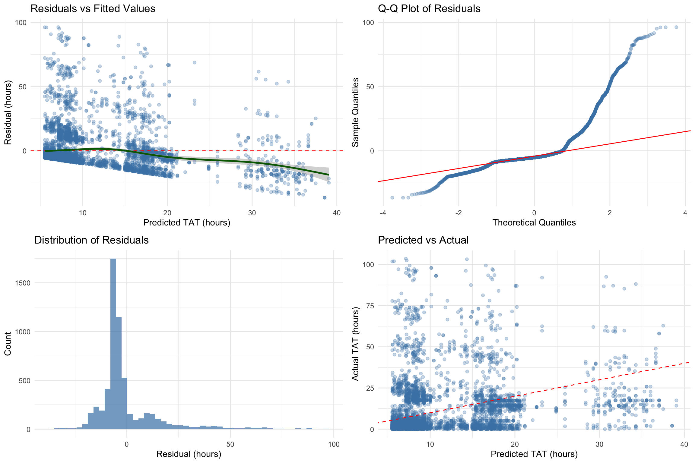
This chapter develops predictive models for turnaround time and forecasts future consultation volumes. TAT prediction is clinically relevant, as the CAP Q-Probes studies have identified key factors influencing turnaround times for complex specimens (Volmar et al. 2015), and recent evaluations have confirmed the utility of TAT as a quality metric in surgical pathology (Sharma et al. 2025).

[1] TRUE

17.1 Predicting Turnaround Time

17.1.1 Feature Engineering

Create features for modeling:

Model Dataset Summary

N_Observations	N_Responders	N_Askers	Mean_TAT	SD_TAT
5882	32	33	10.3	16.1

17.1.2 Linear Regression Model

Linear Regression Coefficients

term	estimate	std.error	statistic	p.value
(Intercept)	1.2521	0.0318	39.4162	0.0000
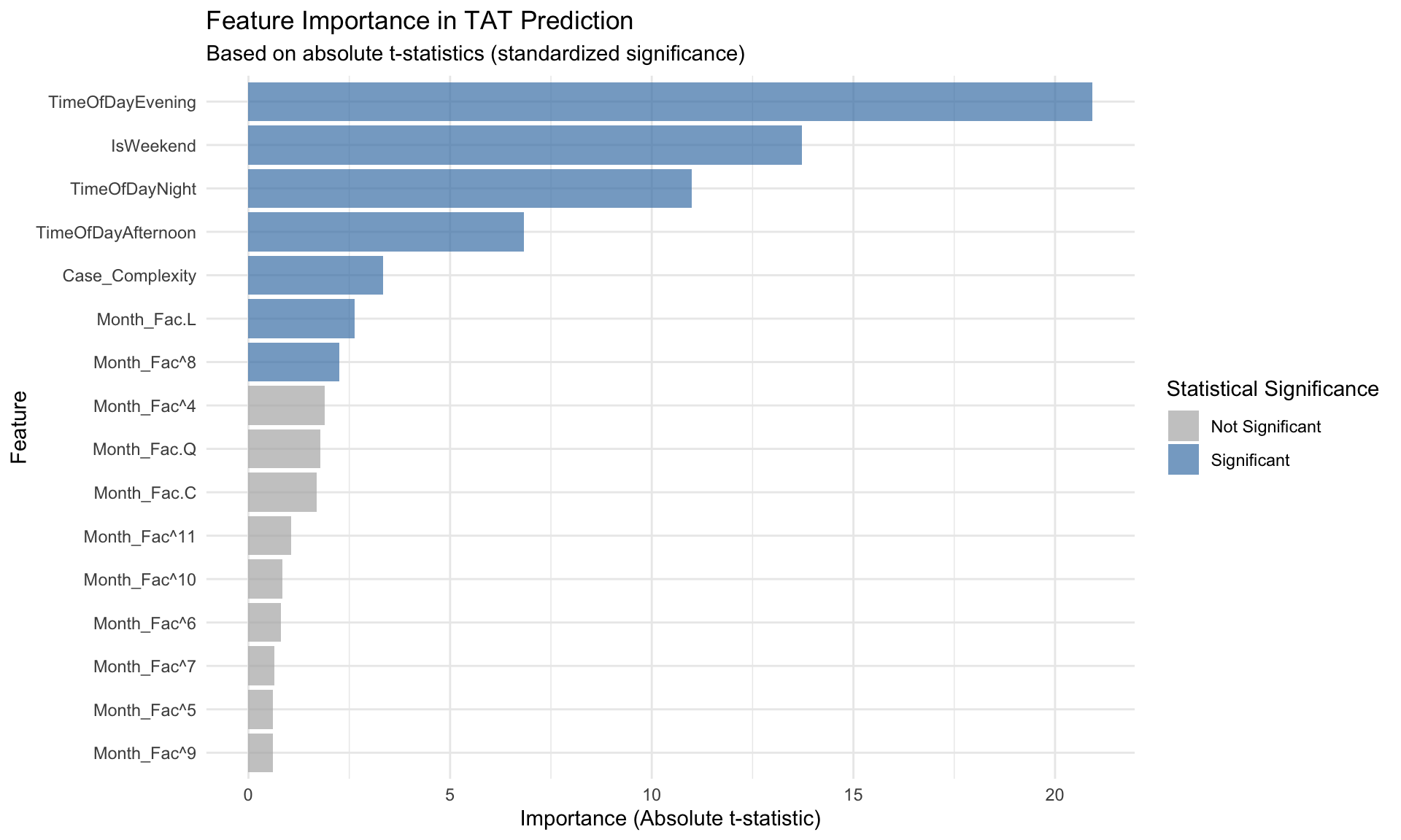
IsWeekend	0.5829	0.0425	13.7260	0.0000
TimeOfDayAfternoon	0.2227	0.0326	6.8281	0.0000
TimeOfDayEvening	0.9208	0.0440	20.9292	0.0000
TimeOfDayNight	0.9010	0.0819	10.9951	0.0000
Month_Fac.L	0.1298	0.0492	2.6382	0.0084
Month_Fac.Q	0.0905	0.0507	1.7855	0.0742
Month_Fac.C	-0.0856	0.0505	-1.6950	0.0901
Month_Fac^4	-0.0939	0.0499	-1.8836	0.0597
Month_Fac^5	0.0303	0.0500	0.6063	0.5443
Month_Fac^6	0.0413	0.0513	0.8058	0.4204
Month_Fac^7	-0.0315	0.0496	-0.6347	0.5256
Month_Fac^8	-0.1126	0.0501	-2.2475	0.0246
Month_Fac^9	-0.0313	0.0524	-0.5978	0.5500
Month_Fac^10	-0.0437	0.0522	-0.8366	0.4028
Month_Fac^11	0.0558	0.0529	1.0538	0.2920
Case_Complexity	0.0396	0.0119	3.3366	0.0009

17.1.3 Model Performance and Cross-Validation

In-sample metrics provide an optimistic upper bound. To estimate out-of-sample performance, we perform 10-fold cross-validation on the linear regression model.

Model Performance Metrics: In-Sample and 10-Fold Cross-Validation

Metric	Value	Interpretation
R-squared (in-sample)	0.1248	12.5% of variance in log(TAT+1) explained
Adjusted R-squared	0.1224	Adjusted for number of predictors (log scale)
RMSE (in-sample, hours)	15.84	Average prediction error on original scale (training)
MAE (in-sample, hours)	10.3	Average absolute error on original scale (training)
R-squared (10-fold CV)	0.1199 +/- 0.0253	Out-of-sample estimate (mean +/- SD across folds)
RMSE (10-fold CV, hours)	15.86 +/- 0.9	Out-of-sample prediction error
MAE (10-fold CV, hours)	10.33 +/- 0.48	Out-of-sample absolute error
Note:
Original-scale predictions use Duan's smearing estimator (factor = 1.9951) to correct for back-transformation bias (Jensen's inequality).

17.1.4 Linear Model Assumption Diagnostics

Linear Regression Assumption Diagnostics

Test	Statistic	P-value	Interpretation
Shapiro-Wilk normality (subsample of 5,000 from 5,882)	0.9703	<2e-16	Residuals non-normal (expected for large N; inference is asymptotically valid)
Breusch-Pagan heteroscedasticity	153.4220	<2e-16	Heteroscedasticity detected -- consider robust standard errors
Max VIF (multicollinearity)	1.0100	Acceptable (< 5)	No multicollinearity concern

17.1.5 Residual Analysis

17.2 Classification Model: Fast vs Slow Response

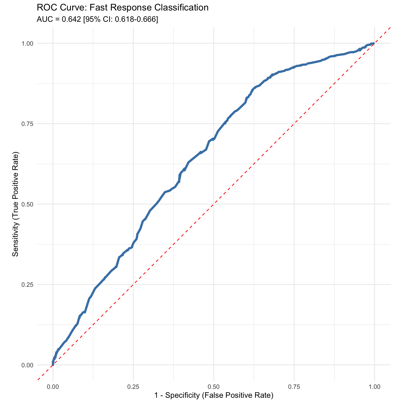
Predict whether a consultation will be completed within 24 hours. The 24-hour threshold is a commonly adopted benchmark for intradepartmental consultation responsiveness, consistent with targets described in CAP laboratory quality literature (Volmar et al. 2015).

Logistic Regression Coefficients (Fast Response Prediction)

term	estimate	std.error	statistic	p.value
(Intercept)	2.4048	0.0977	24.6036	0.0000
IsWeekend	-1.3695	0.0954	-14.3563	0.0000
TimeOfDayAfternoon	-0.1197	0.0975	-1.2273	0.2197
TimeOfDayEvening	-0.1882	0.1239	-1.5186	0.1289
TimeOfDayNight	0.6736	0.3124	2.1565	0.0310
Month_Fac.L	0.0698	0.1466	0.4765	0.6337
Month_Fac.Q	0.1750	0.1546	1.1320	0.2576
Month_Fac.C	-0.0324	0.1505	-0.2152	0.8296
Month_Fac^4	0.3084	0.1479	2.0853	0.0370
Month_Fac^5	-0.1182	0.1467	-0.8054	0.4206
Month_Fac^6	-0.0618	0.1475	-0.4191	0.6751
Month_Fac^7	0.0125	0.1437	0.0872	0.9305
Month_Fac^8	0.0447	0.1442	0.3099	0.7566
Month_Fac^9	-0.0699	0.1490	-0.4689	0.6392
Month_Fac^10	0.1353	0.1515	0.8935	0.3716
Month_Fac^11	-0.2553	0.1572	-1.6242	0.1043
Case_Complexity	0.0149	0.0347	0.4305	0.6668

17.2.1 Classification Performance

Note: As with the linear model above, classification metrics are in-sample estimates. The AUC, sensitivity, and specificity reported here are likely overfitted to the training data.

Classification Model Performance

Metric	Value	Percentage
Accuracy	0.8886	88.86%
Sensitivity (Recall)	1.0000	100%
Specificity	0.0000	0%
Precision	0.8886	88.86%

Confusion Matrix

	Predicted
	0	1
0	0	655
1	0	5227

17.2.2 Logistic Model Diagnostics

Logistic Regression Model Diagnostics and Cross-Validation

Metric	Value	Interpretation
McFadden's pseudo-R2	0.052	Poor fit (< 0.1)
Hosmer-Lemeshow goodness-of-fit	chi2 = 7.05, p = 0.531	Adequate calibration (fail to reject H0: good fit)
AIC	3929.9	Lower is better; penalizes model complexity
Accuracy (10-fold CV)	88.9% +/- 1.3%	Out-of-sample classification accuracy (mean +/- SD)
AUC (10-fold CV)	0.609 +/- 0.024	Out-of-sample discriminative ability

17.2.3 ROC Curve

17.3 Time Series Forecasting

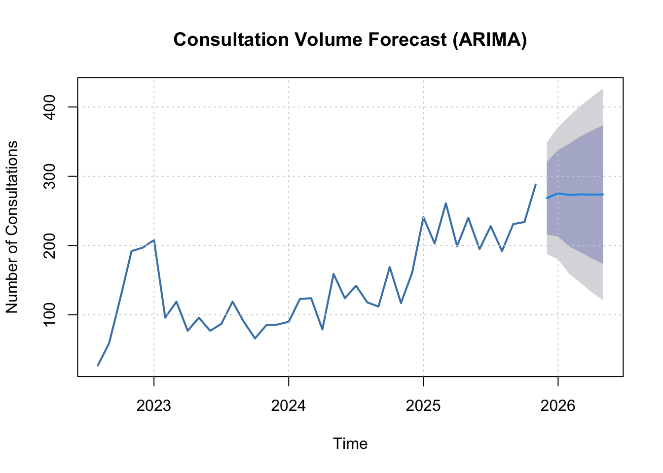
17.3.1 Forecasting Consultation Volume

6-Month Consultation Volume Forecast

	Point Forecast	Lo 80	Hi 80	Lo 95	Hi 95	Month
Dec 2025	268.49	215.87	321.11	188.02	348.96	2025-12-01
Jan 2026	275.54	213.11	337.97	180.05	371.02	2026-01-01
Feb 2026	272.99	198.59	347.40	159.20	386.78	2026-02-01
Mar 2026	273.91	190.37	357.46	146.14	401.68	2026-03-01
Apr 2026	273.58	181.43	365.73	132.64	414.51	2026-04-01
May 2026	273.70	173.80	373.60	120.92	426.48	2026-05-01

17.3.2 ARIMA Model Diagnostics

ARIMA Model Diagnostics

Diagnostic	Value	Interpretation
ARIMA order: 1,1,0	ARIMA(1,1,0)	Selected by auto.arima via AICc
Residual autocorrelation (Ljung-Box)	Q = 8.06, p = 0.623	No significant residual autocorrelation -- model adequately captures temporal structure
Residual normality (Shapiro-Wilk)	W = 0.9728, p = 0.44	Residuals approximately normal -- prediction intervals valid
Residual mean	8.341	Should be near zero for unbiased forecasts
Residual SD	39.64	Forecast uncertainty scale

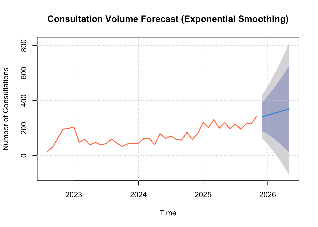
17.3.3 Exponential Smoothing

Forecasting Model Comparison (In-Sample Accuracy and Residual Diagnostics)

Model	Type	RMSE	MAE	MAPE	Ljung-Box p
ARIMA	ARIMA(1,1,0)	40.02	30.44	22.81	0.623
Exponential Smoothing (ETS)	ETS(M,A,N)	43.55	32.86	25.25	0.934

17.4 Feature Importance Analysis

17.4.1 Variable Importance in TAT Prediction

17.5 Model Recommendations

Predictive Modeling Recommendations

Finding	Recommendation
Weekend consultations have longer TAT	Consider weekend-specific resource allocation or expectations
Model explains only 12.5% of variance	Consider additional features: responder workload, case type, subspecialty

17.6 Model Summary

Summary of Predictive Models

Model	Target Variable	Key Metric	Use Case
Linear Regression (TAT Prediction)	Log(TAT + 1)	R² = 0.125	Estimate expected turnaround time
Logistic Regression (Fast Response)	Within 24 hours (Binary)	Accuracy = 88.9%	Identify consultations at risk of delay
ARIMA (Volume Forecast)	Monthly consultation count	RMSE = 40.02	Forecast future consultation demand
Exponential Smoothing	Monthly consultation count	RMSE = 43.55	Alternative forecasting approach

Sharma, Anuradha, Vemuri Nishadham, Prerna Gupta, Gaurav Gupta, Deveshi Sharma, Shivani Goel, Sanjay Pasricha, Mehar Kamboj, and Ashim Mehta. 2025. “Evaluation of Turnaround Times of Diagnostic Biopsies: A Metric of Quality in Surgical Pathology.” International Journal of Surgical Pathology. https://doi.org/10.1177/10668969241261561.

Volmar, Keith E., Michael O. Idowu, Paul F. Engstrom, and Paolo Gattuso. 2015. “Turnaround Time for Large or Complex Specimens in Surgical Pathology: A College of American Pathologists q-Probes Study of 56 Institutions.” Archives of Pathology & Laboratory Medicine 139 (2): 171–77. https://doi.org/10.5858/arpa.2013-0671-CP.