9 Network Analysis
Consultation networks reveal how expertise flows between pathologists and can identify key knowledge brokers within a department (Goebel, Ettler, and Walsh 2018). Understanding these patterns is essential for optimizing resource allocation and ensuring that consultation requests reach the most appropriate experts (Renshaw et al. 2002). Social network analysis (SNA) has been increasingly applied to study professional advice and collaboration patterns among healthcare providers, with directed and weighted graphs serving as natural representations of referral and consultation relationships (Sabot et al. 2017; Biscione and Domingues da Silva 2024). In physician networks, centrality measures such as betweenness centrality have been shown to correlate with healthcare costs and care intensity, demonstrating the practical significance of network topology (Barnett et al. 2012; Landon et al. 2012). Digital pathology platforms, including telepathology consultation networks, have expanded the possibilities for intradepartmental and inter-institutional collaboration (Chong et al. 2019).
9.1 Anonymized Consultation Network
9.1.1 Network Graph (igraph)
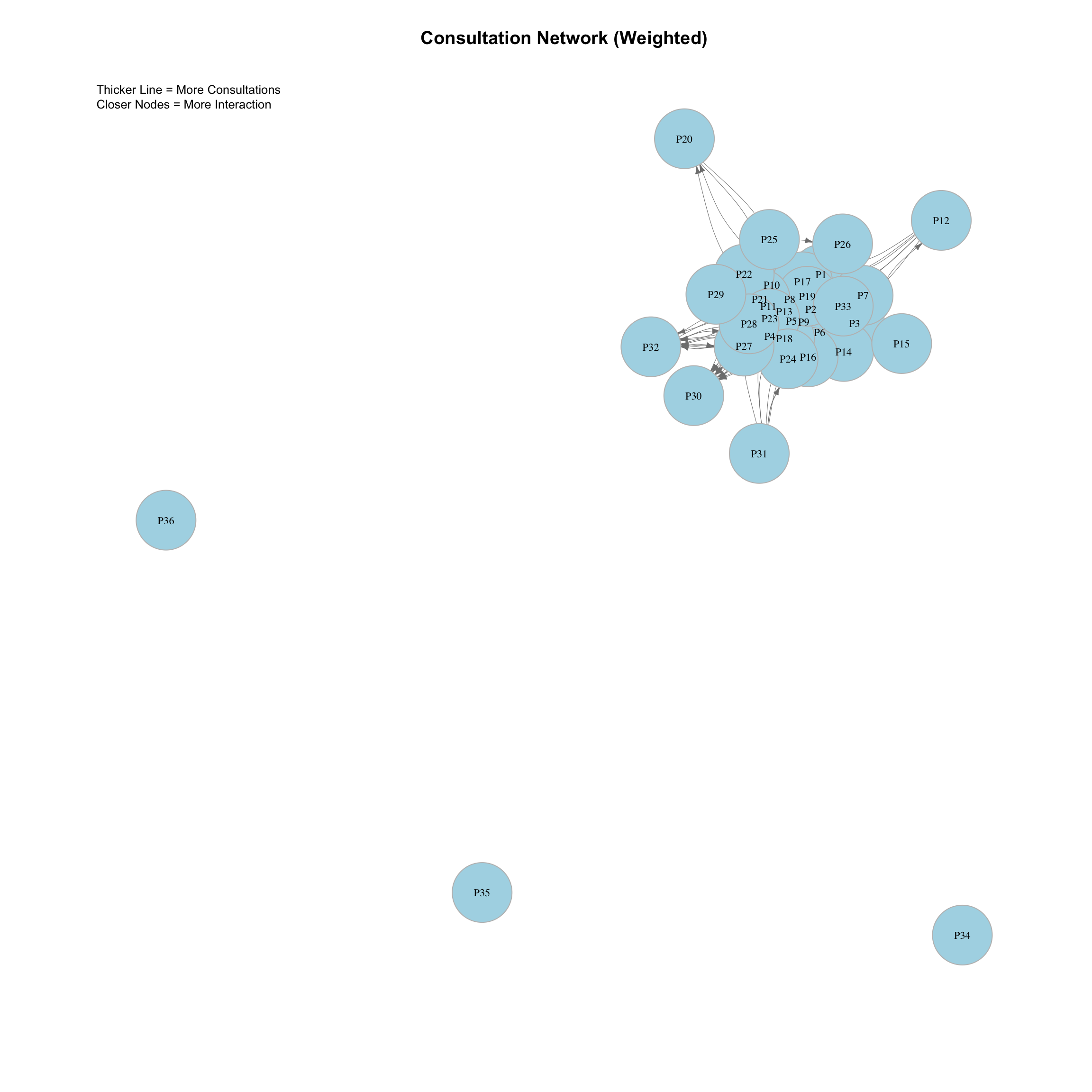
This graph visualizes the consultation network. - Node: Pathologist. - Arrow: Direction of consultation (Asker -> Responder). - Line Thickness: Proportional to the number of consultations (Thicker = More). - Proximity: Nodes with more interactions are pulled closer together.
9.1.2 Circular Plot (DescTools)
This circular plot shows the flow of consultations. - Segments: Pathologists. - Links: Consultations moving from Asker to Responder. - Width of Link: Number of consultations.
9.2 Publication-Quality Chord Diagrams
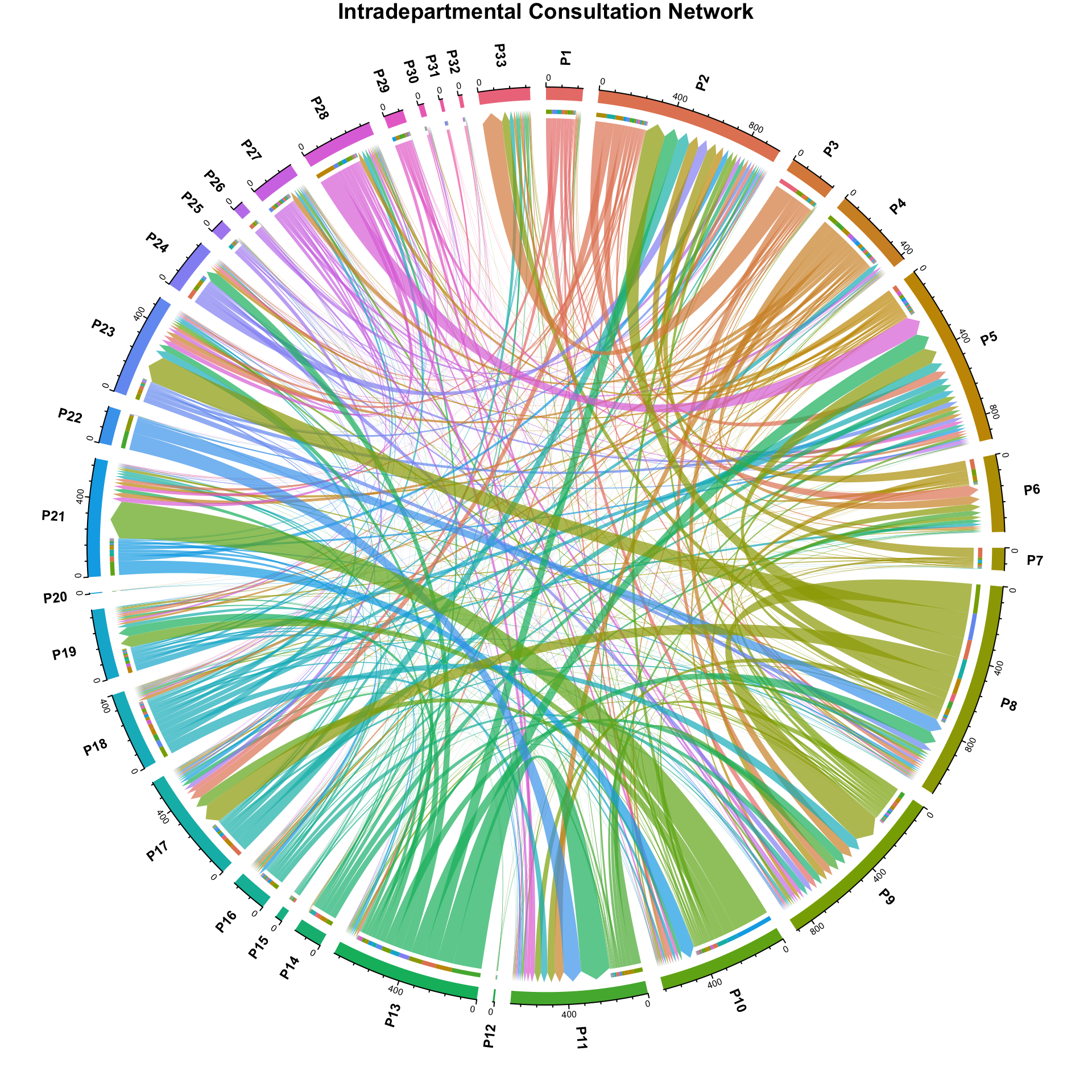
Chord diagrams provide an intuitive, publication-ready visualization of directed flows between entities arranged around a circle. Unlike the basic circular plot above, the circlize implementation offers precise control over color mapping, gap sizes, label placement, and directional ribbon rendering – all critical for conference presentations. In a chord diagram, each segment on the circle represents a pathologist (or category), the width of the segment is proportional to total consultation volume, and the ribbons connecting segments represent flows from Asker to Responder. Wider ribbons indicate more consultations along that pathway. The direction of the flow is encoded by which end of the ribbon is narrower (origin) versus wider (destination), though in practice both ends are typically read from the labels.
These diagrams were designed for the ECDP/ESDIP 2025 presentation and are intended to be directly usable in slides and posters.
9.2.1 Overall Consultation Flow
This chord diagram shows the complete pathologist-to-pathologist consultation network. Each segment represents a pathologist, and ribbons show the direction and volume of consultations between them.
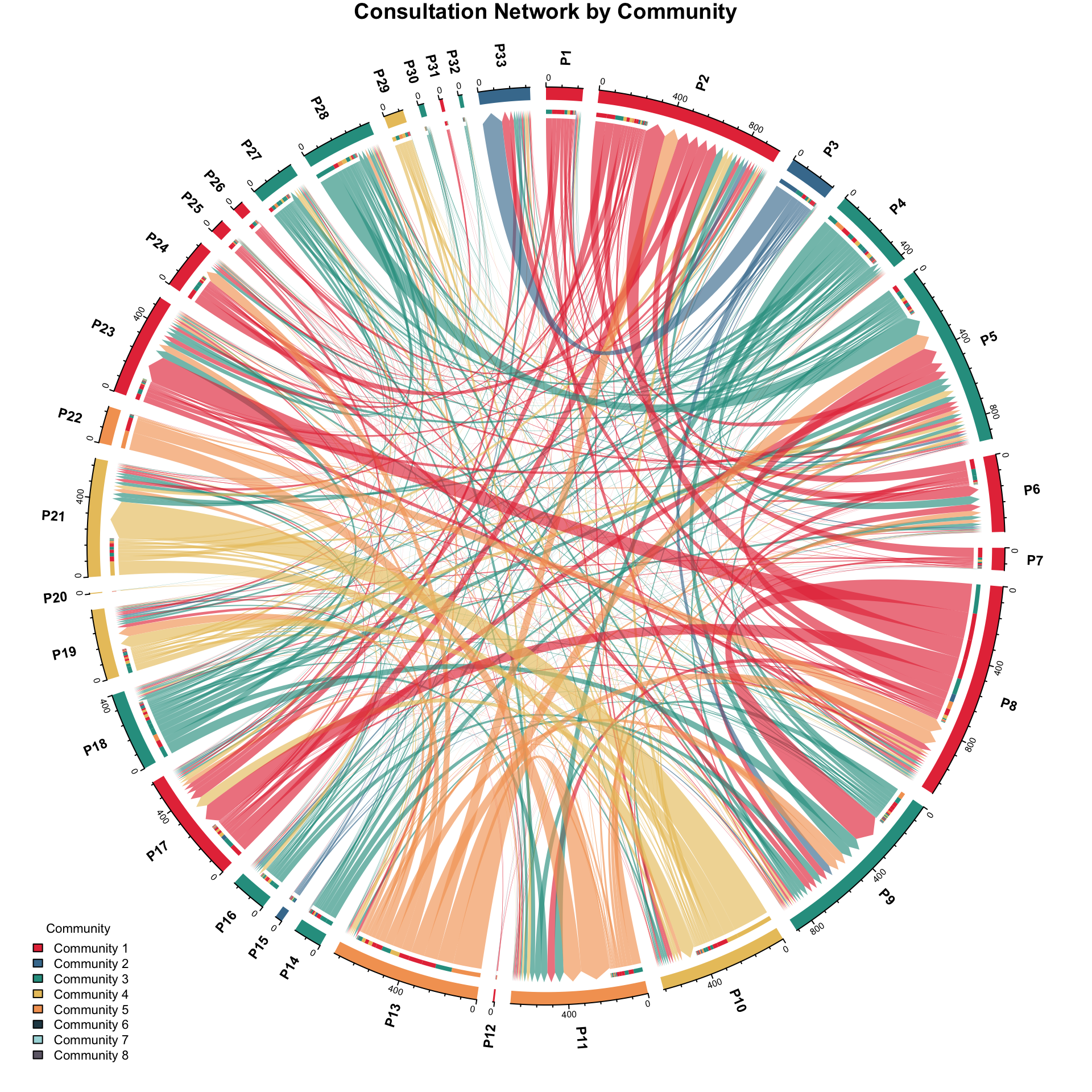
9.2.2 Consultation Flow by Community
This variant colors both segments and ribbons according to the Louvain community membership identified in the community detection analysis below (Section 9.5). Pathologists in the same community share the same color, making it easy to see within-community versus between-community consultation patterns.
9.2.3 Consultation Flow by Question Category
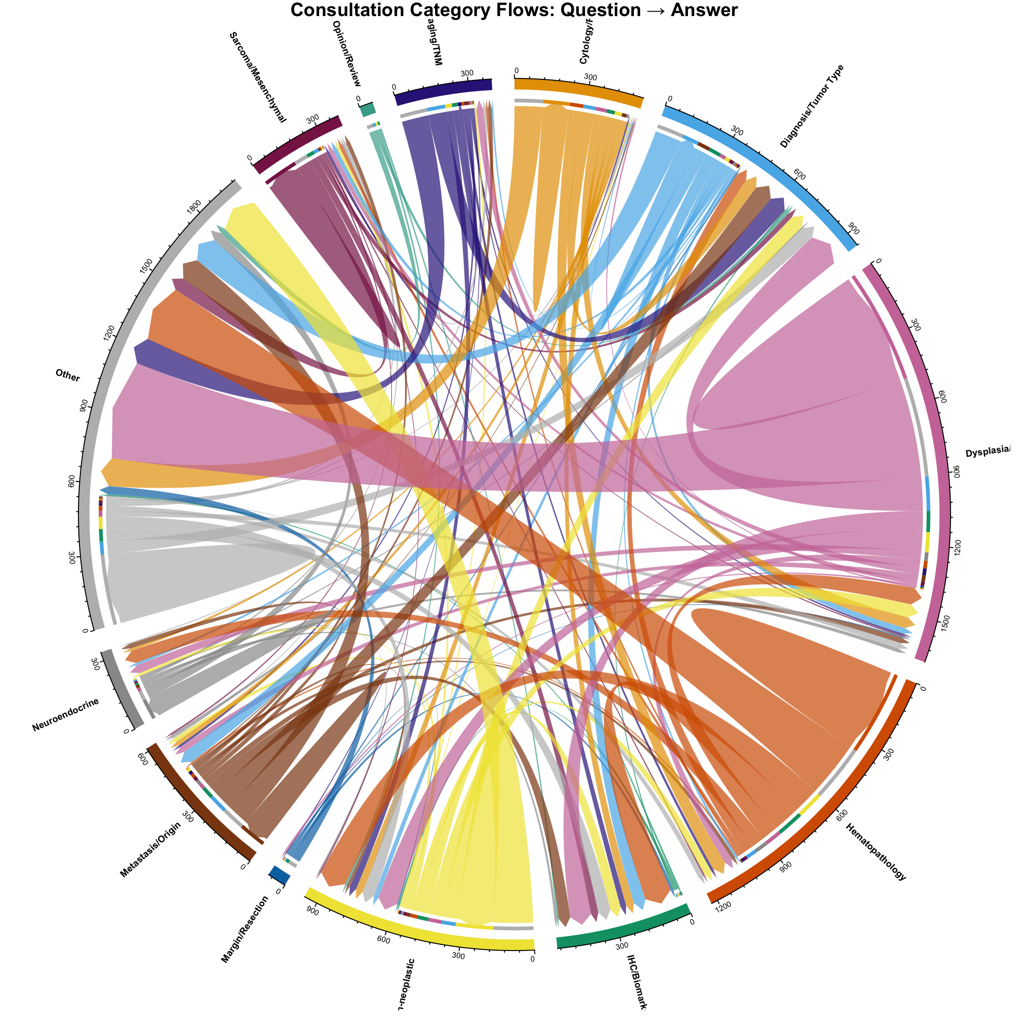
Rather than showing pathologist-to-pathologist flows, this chord diagram visualizes how consultation categories flow between Asker and Responder roles. Each segment represents a consultation category, and ribbons show how many consultations of each question category were answered in each answer category. This reveals diagnostic category shifts – cases where the consultation question is in one domain but the expert response falls in another.
TipReading Chord Diagrams
For the pathologist flow diagrams: Each colored segment on the circle represents one pathologist. The width of the segment reflects their total consultation volume (both sent and received). Ribbons connect pairs of pathologists, with width proportional to the number of consultations between them. The directional arrows on ribbons indicate the flow from Asker to Responder.
For the category flow diagram: Each segment is a consultation category. The dominant self-linking ribbons (same color at both ends) represent cases where the question and answer belong to the same diagnostic category. Cross-category ribbons highlight diagnostic shifts where the expert reclassified the case into a different domain.
Presentation note: These diagrams are formatted for direct use in ECDP/ESDIP conference presentations. For best results in slides, use the HTML output version which preserves high-resolution vector graphics.
9.3 Network Centrality Metrics
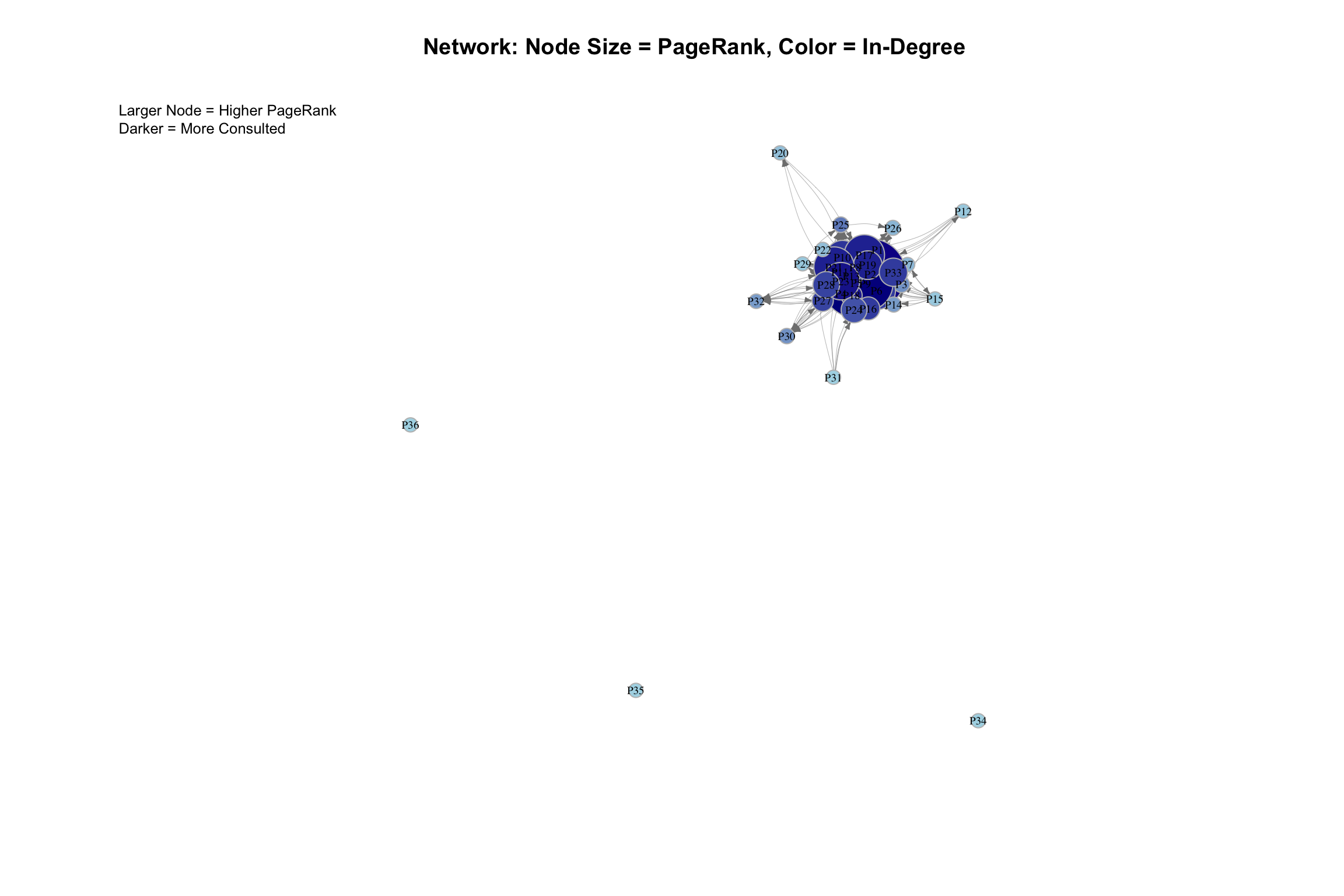
Understanding which pathologists are most central to the consultation network.
| Pathologist | In_Degree | Out_Degree | Total_Degree | In_Strength | Out_Strength | Betweenness | Closeness | Eigenvector | PageRank |
|---|---|---|---|---|---|---|---|---|---|
| P2 | 26 | 20 | 46 | 684 | 275 | 266.00 | 0.3717 | 0.976 | 0.1150 |
| P5 | 29 | 19 | 48 | 751 | 176 | 252.00 | 0.3643 | 1.000 | 0.1136 |
| P9 | 28 | 22 | 50 | 696 | 194 | 132.67 | 0.3832 | 0.720 | 0.0850 |
| P17 | 22 | 16 | 38 | 362 | 207 | 141.00 | 0.3675 | 0.601 | 0.0559 |
| P21 | 22 | 17 | 39 | 399 | 197 | 76.00 | 0.3108 | 0.601 | 0.0559 |
| P8 | 27 | 17 | 44 | 348 | 754 | 117.00 | 0.3942 | 0.370 | 0.0538 |
| P6 | 18 | 13 | 31 | 254 | 136 | 27.00 | 0.3212 | 0.479 | 0.0508 |
| P23 | 24 | 16 | 40 | 407 | 116 | 20.50 | 0.3697 | 0.520 | 0.0503 |
| P11 | 25 | 18 | 43 | 521 | 171 | 39.00 | 0.3561 | 0.406 | 0.0480 |
| P10 | 19 | 20 | 39 | 216 | 434 | 88.00 | 0.3212 | 0.366 | 0.0431 |
| P19 | 22 | 16 | 38 | 227 | 131 | 94.00 | 0.3179 | 0.286 | 0.0333 |
| P33 | 18 | 0 | 18 | 261 | 0 | 0.00 | 0.3124 | 0.267 | 0.0325 |
| P28 | 17 | 18 | 35 | 124 | 241 | 53.50 | 0.3341 | 0.188 | 0.0294 |
| P24 | 15 | 9 | 24 | 120 | 140 | 31.00 | 0.3195 | 0.197 | 0.0279 |
| P16 | 18 | 15 | 33 | 75 | 111 | 0.00 | 0.2767 | 0.147 | 0.0223 |
| P13 | 14 | 20 | 34 | 68 | 684 | 39.00 | 0.3683 | 0.156 | 0.0215 |
| P27 | 17 | 18 | 35 | 94 | 133 | 56.00 | 0.2534 | 0.099 | 0.0191 |
| P18 | 23 | 24 | 47 | 82 | 319 | 53.67 | 0.3226 | 0.094 | 0.0189 |
| P4 | 19 | 25 | 44 | 79 | 345 | 12.00 | 0.3316 | 0.059 | 0.0151 |
| P1 | 7 | 17 | 24 | 28 | 158 | 30.00 | 0.2824 | 0.049 | 0.0099 |
| P3 | 7 | 13 | 20 | 14 | 228 | 30.00 | 0.2987 | 0.030 | 0.0092 |
| P25 | 10 | 12 | 22 | 17 | 56 | 0.00 | 0.2457 | 0.019 | 0.0080 |
| P30 | 7 | 8 | 15 | 18 | 11 | 0.00 | 0.1279 | 0.014 | 0.0077 |
| P14 | 6 | 12 | 18 | 8 | 139 | 0.00 | 0.2934 | 0.012 | 0.0071 |
| P26 | 3 | 9 | 12 | 6 | 50 | 0.00 | 0.2440 | 0.018 | 0.0070 |
| P32 | 6 | 7 | 13 | 8 | 12 | 0.00 | 0.0770 | 0.005 | 0.0060 |
| P7 | 3 | 14 | 17 | 3 | 111 | 0.00 | 0.3043 | 0.002 | 0.0057 |
| P22 | 2 | 6 | 8 | 3 | 185 | 0.00 | 0.3478 | 0.001 | 0.0056 |
| P15 | 1 | 12 | 13 | 1 | 37 | 0.00 | 0.1560 | 0.000 | 0.0054 |
| P20 | 2 | 2 | 4 | 2 | 3 | 0.00 | 0.0554 | 0.002 | 0.0054 |
| P29 | 1 | 12 | 13 | 1 | 99 | 0.00 | 0.2366 | 0.000 | 0.0054 |
| P12 | 1 | 6 | 7 | 1 | 8 | 0.00 | 0.0550 | 0.000 | 0.0053 |
| P31 | 0 | 6 | 6 | 0 | 17 | 0.00 | 0.1605 | 0.000 | 0.0053 |
| P34 | 0 | 0 | 0 | 0 | 0 | 0.00 | NaN | 0.000 | 0.0053 |
| P35 | 0 | 0 | 0 | 0 | 0 | 0.00 | NaN | 0.000 | 0.0053 |
| P36 | 0 | 0 | 0 | 0 | 0 | 0.00 | NaN | 0.000 | 0.0053 |
9.3.1 Interpretation of Centrality Metrics
Centrality metrics capture different aspects of a pathologist’s role in the consultation network. These measures have been applied to physician referral networks to identify key opinion leaders and potential bottlenecks (Chong et al. 2019). Studies of patient-sharing physician networks have demonstrated that network structure – particularly the centrality of primary care providers – is significantly associated with resource utilization, with higher betweenness centrality linked to lower costs and fewer specialist visits (Barnett et al. 2012).
- In-Degree: Number of unique pathologists who sought consultation from this expert. High in-degree = broadly sought-after expert.
- Out-Degree: Number of unique pathologists this person consulted. High out-degree = broadly seeking input.
- In-Strength: Total number of consultations received (weighted in-degree). High in-strength = highest consultation volume.
- Out-Strength: Total number of consultations initiated (weighted out-degree). High out-strength = highest request volume.
- Betweenness: How often a pathologist lies on the shortest path between others. High betweenness = broker/bridge.
- Closeness: How quickly a pathologist can reach others. High closeness = efficient communicator.
- Eigenvector: Importance based on connections to other important nodes. High eigenvector = connected to key players.
- PageRank: Google’s algorithm - considers both quantity and quality of connections.
9.3.2 Top Experts (By Total Consultations Received)
Pathologists with the highest consultation volume:
| Pathologist | Total Consultations | Unique Askers | PageRank | Eigenvector |
|---|---|---|---|---|
| P5 | 751 | 29 | 0.1136 | 1.000 |
| P9 | 696 | 28 | 0.0850 | 0.720 |
| P2 | 684 | 26 | 0.1150 | 0.976 |
| P11 | 521 | 25 | 0.0480 | 0.406 |
| P23 | 407 | 24 | 0.0503 | 0.520 |
| P21 | 399 | 22 | 0.0559 | 0.601 |
| P17 | 362 | 22 | 0.0559 | 0.601 |
| P8 | 348 | 27 | 0.0538 | 0.370 |
| P33 | 261 | 18 | 0.0325 | 0.267 |
| P6 | 254 | 18 | 0.0508 | 0.479 |
9.3.3 Top Askers (By Total Consultations Initiated)
Pathologists who initiate the most consultations:
| Pathologist | Total Requests | Unique Responders |
|---|---|---|
| P8 | 754 | 17 |
| P13 | 684 | 20 |
| P10 | 434 | 20 |
| P4 | 345 | 25 |
| P18 | 319 | 24 |
| P2 | 275 | 20 |
| P28 | 241 | 18 |
| P3 | 228 | 13 |
| P17 | 207 | 16 |
| P21 | 197 | 17 |
9.4 Centrality Visualization
9.5 Community Detection
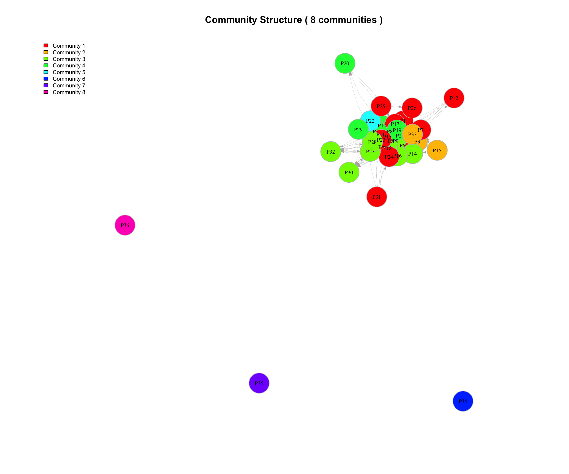
Identifying clusters or subgroups within the consultation network. Community structure in consultation networks often reflects subspecialty expertise, with pathologists who share case types forming tightly connected groups (Goebel, Ettler, and Walsh 2018).
| Algorithm | Communities | Modularity |
|---|---|---|
| Louvain | 8 | 0.173 |
| Walktrap | 6 | 0.115 |
| Edge Betweenness | 21 | 0.003 |
| Fast Greedy | 8 | 0.175 |
Note: Higher modularity indicates stronger community structure. We’ll use the algorithm with the highest modularity for further analysis.
9.5.1 Community Membership (Louvain Method)
| Pathologist | Community | In_Degree | Out_Degree |
|---|---|---|---|
| P8 | 1 | 27 | 17 |
| P2 | 1 | 26 | 20 |
| P23 | 1 | 24 | 16 |
| P17 | 1 | 22 | 16 |
| P6 | 1 | 18 | 13 |
| P24 | 1 | 15 | 9 |
| P25 | 1 | 10 | 12 |
| P1 | 1 | 7 | 17 |
| P7 | 1 | 3 | 14 |
| P26 | 1 | 3 | 9 |
| P12 | 1 | 1 | 6 |
| P31 | 1 | 0 | 6 |
| P33 | 2 | 18 | 0 |
| P3 | 2 | 7 | 13 |
| P15 | 2 | 1 | 12 |
| P5 | 3 | 29 | 19 |
| P9 | 3 | 28 | 22 |
| P18 | 3 | 23 | 24 |
| P4 | 3 | 19 | 25 |
| P16 | 3 | 18 | 15 |
| P27 | 3 | 17 | 18 |
| P28 | 3 | 17 | 18 |
| P30 | 3 | 7 | 8 |
| P14 | 3 | 6 | 12 |
| P32 | 3 | 6 | 7 |
| P19 | 4 | 22 | 16 |
| P21 | 4 | 22 | 17 |
| P10 | 4 | 19 | 20 |
| P20 | 4 | 2 | 2 |
| P29 | 4 | 1 | 12 |
| P11 | 5 | 25 | 18 |
| P13 | 5 | 14 | 20 |
| P22 | 5 | 2 | 6 |
| P34 | 6 | 0 | 0 |
| P35 | 7 | 0 | 0 |
| P36 | 8 | 0 | 0 |
9.5.2 Community Visualization
9.5.3 Community Summary Statistics
| Community | N_Members | Total_In_Degree | Total_Out_Degree | Avg_In_Degree | Avg_Out_Degree |
|---|---|---|---|---|---|
| 1 | 12 | 156 | 155 | 13.0 | 12.9 |
| 3 | 10 | 170 | 168 | 17.0 | 16.8 |
| 4 | 5 | 66 | 67 | 13.2 | 13.4 |
| 2 | 3 | 26 | 25 | 8.7 | 8.3 |
| 5 | 3 | 41 | 44 | 13.7 | 14.7 |
| 6 | 1 | 0 | 0 | 0.0 | 0.0 |
| 7 | 1 | 0 | 0 | 0.0 | 0.0 |
| 8 | 1 | 0 | 0 | 0.0 | 0.0 |
| Community | N_Members | Dominant_Subspecialties | Common_Organs | Common_Topics |
|---|---|---|---|---|
| 1 | 12 | General (33%), GIS (25%), BST (17%) | TIROID (10%), Kolon (9%), Mide (5%) | Dysplasia/Grade (19%), Hematopathology (12%), Other (11%) |
| 3 | 10 | General (30%), GIS (20%), Hemato (20%), Lung (20%) | MIDE BIOPSI (12%), Kolon (11%), KOLON BIOPSI (11%) | Hematopathology (30%), Dysplasia/Grade (26%), Inflammatory/Non-neoplastic (10%) |
| 4 | 5 | General (40%), Gyn (40%), Breast (20%) | MEME (16%), UTERUS (11%), Endometrium (6%) | Dysplasia/Grade (24%), Metastasis/Origin (16%), Other (14%) |
| 2 | 3 | General (67%), NA (33%) | TIROID (16%), Kolon (9%), DERI (8%) | Dysplasia/Grade (21%), Inflammatory/Non-neoplastic (12%), Diagnosis/Tumor Type (11%) |
| 5 | 3 | General (33%), Pancreas (33%), Uro (33%) | Mide (23%), Kolon (20%), MIDE BIOPSI (9%) | Dysplasia/Grade (32%), Hematopathology (26%), Metastasis/Origin (11%) |
| 6 | 1 | General (100%) | NA | NA |
| 7 | 1 | General (100%) | NA | NA |
| 8 | 1 | General (100%) | NA | NA |
9.6 Network Density and Reciprocity
Global network properties:
| Property | Value | Interpretation |
|---|---|---|
| Network Density | 0.3643 | 36.43% of all possible connections exist |
| Reciprocity | 0.5249 | 52.49% of connections are reciprocated |
| Global Clustering Coefficient | 0.7265 | Probability that neighbors of a node are connected |
| Average Path Length | 2.9400 | Average steps between any two pathologists |
| Network Diameter | 8.0000 | Maximum steps needed to connect any two pathologists |
9.7 Reciprocity Analysis
Examining bidirectional consultation relationships:
| From | To | Weight_From_To | Weight_To_From | Total |
|---|---|---|---|---|
| P10 | P21 | 197 | 74 | 271 |
| P8 | P23 | 142 | 32 | 174 |
| P8 | P9 | 155 | 4 | 159 |
| P11 | P13 | 5 | 154 | 159 |
| P5 | P28 | 22 | 104 | 126 |
| P8 | P17 | 105 | 14 | 119 |
| P2 | P8 | 12 | 106 | 118 |
| P2 | P6 | 56 | 53 | 109 |
| P2 | P17 | 45 | 62 | 107 |
| P5 | P8 | 4 | 87 | 91 |
9.8 Temporal Network Evolution
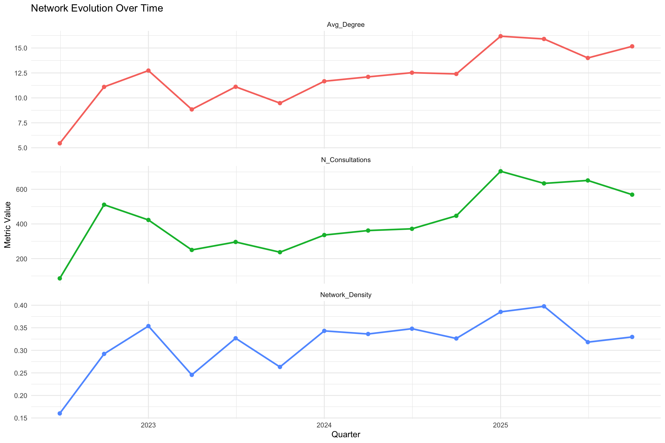
How has the network structure changed over time? Note that quarterly network slices with few consultations may produce unstable centrality metrics. Quarters with fewer than 10 edges should be interpreted with caution.
9.9 Consultation Categories and Network Structure
9.9.1 Category-Weighted Network
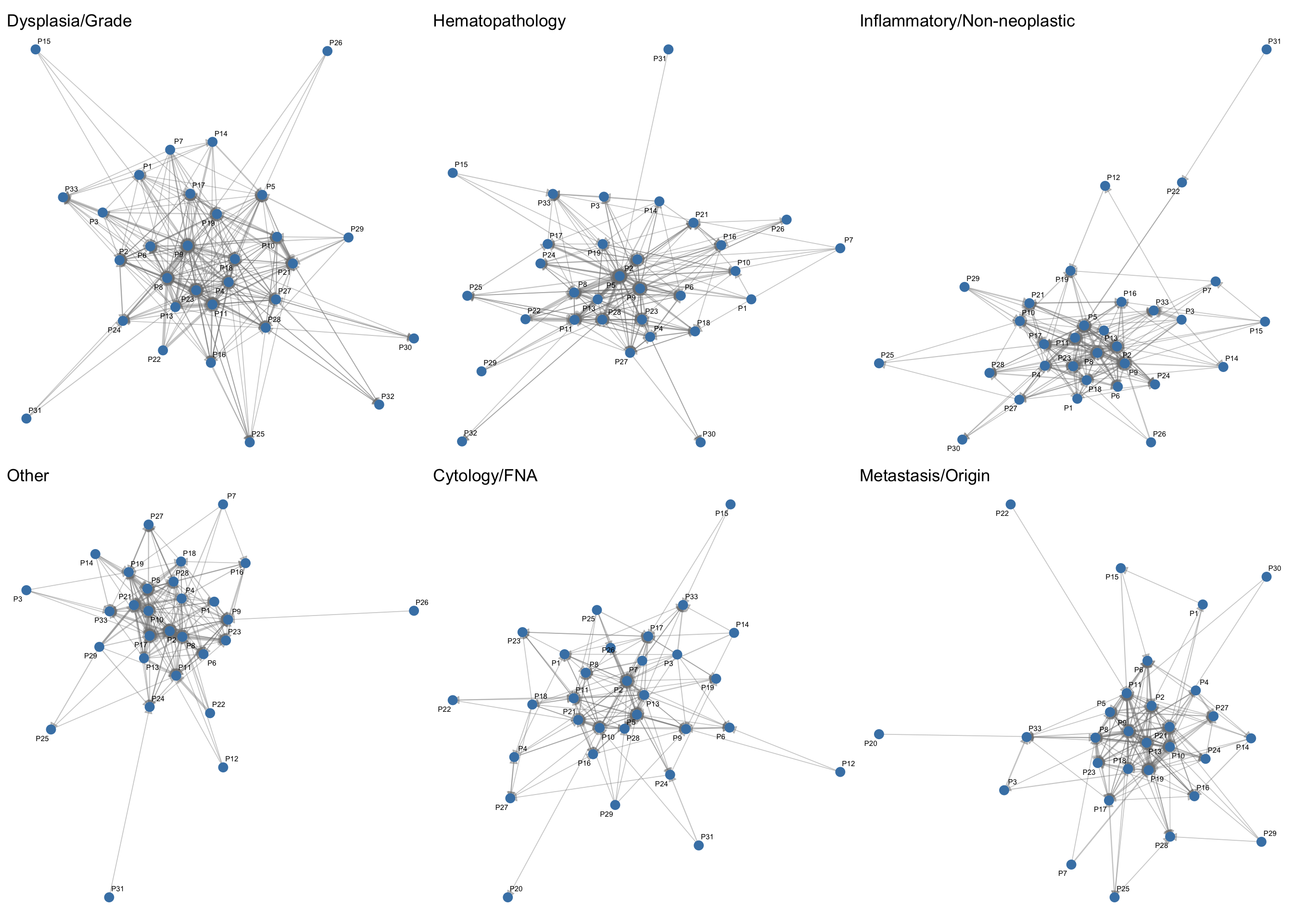
How do consultation topics shape the network? This section examines category-specific subnetworks to reveal topic-dependent interaction patterns.
9.9.2 Topic Specialization by Network Position
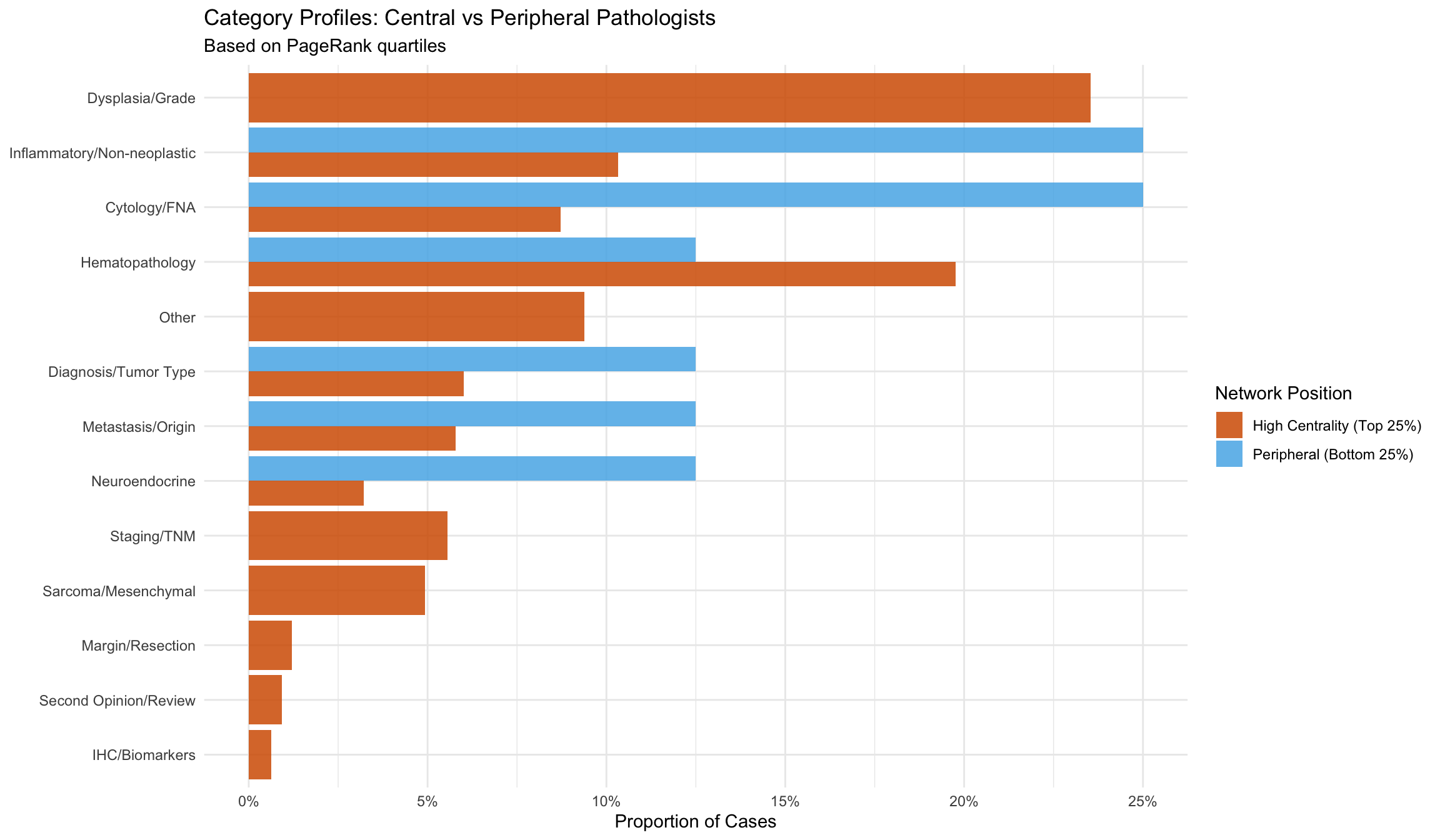
Do central pathologists handle different types of consultations than peripheral ones?
9.9.3 Category Flow: Question to Answer
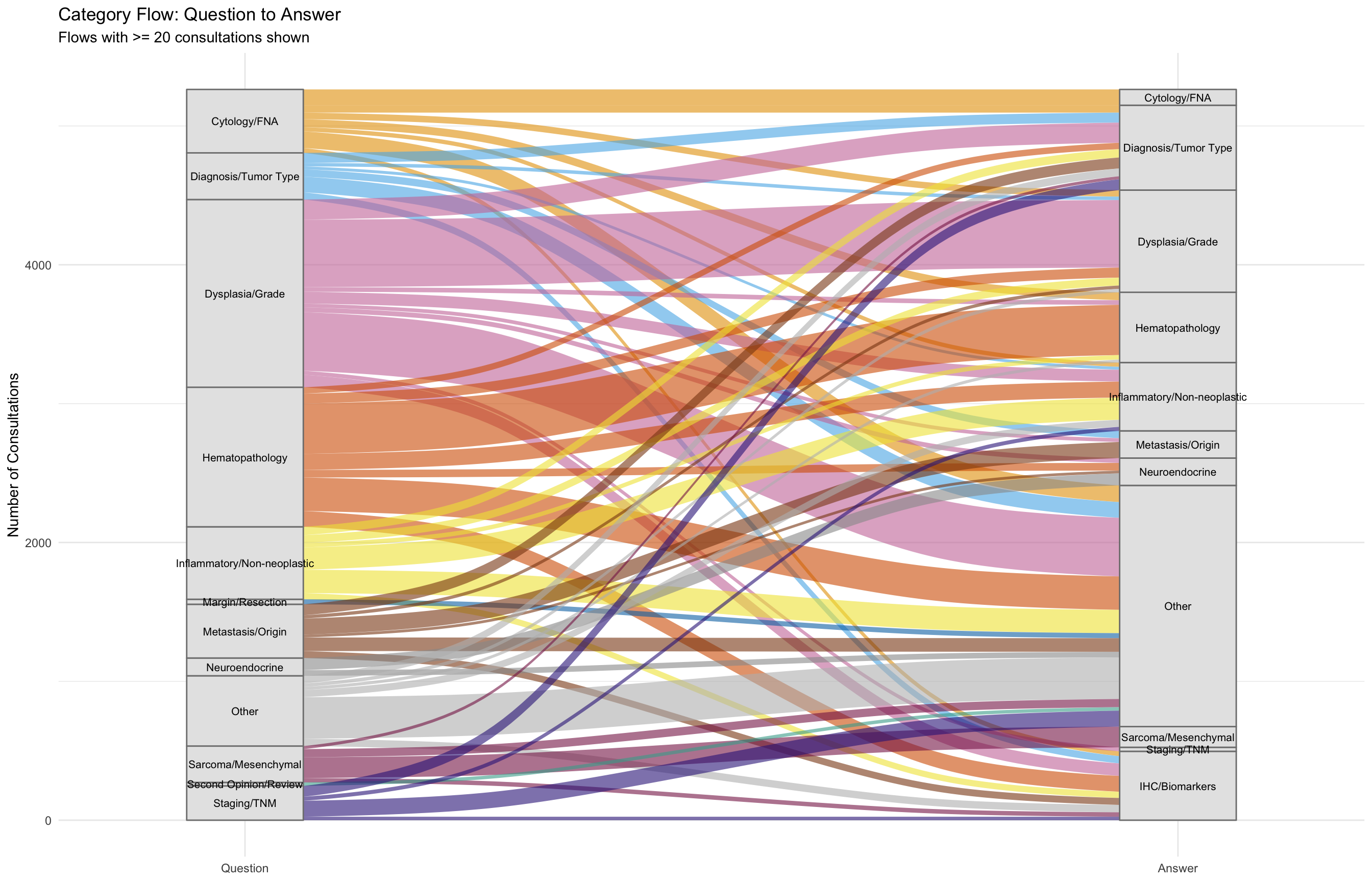
How often does the answer category differ from the question category? This alluvial diagram traces the flow from question topics to answer topics.
| Question Category | Total | Same Answer | Shifted | % Same |
|---|---|---|---|---|
| Dysplasia/Grade | 1385 | 486 | 899 | 35.1 |
| Hematopathology | 1040 | 362 | 678 | 34.8 |
| Inflammatory/Non-neoplastic | 578 | 160 | 418 | 27.7 |
| Other | 549 | 299 | 250 | 54.5 |
| Cytology/FNA | 493 | 114 | 379 | 23.1 |
| Metastasis/Origin | 458 | 116 | 342 | 25.3 |
| Diagnosis/Tumor Type | 391 | 72 | 319 | 18.4 |
| Staging/TNM | 318 | 16 | 302 | 5.0 |
| Sarcoma/Mesenchymal | 296 | 149 | 147 | 50.3 |
| Neuroendocrine | 192 | 87 | 105 | 45.3 |
| Margin/Resection | 75 | 1 | 74 | 1.3 |
| Second Opinion/Review | 69 | 1 | 68 | 1.4 |
| IHC/Biomarkers | 38 | 8 | 30 | 21.1 |
**Overall concordance:** 31.8% of consultations retain the same category between question and answer. 68.2% involve a category shift.9.10 Network Isolate Detection
A critical safety function of network analysis in remote digital pathology is the identification of potential network “isolates” — pathologists with both low in-degree (rarely consulted) and low out-degree (rarely seeking consultation) who may be working in silos, disconnected from the department’s quality assurance web (Goebel, Ettler, and Walsh 2018). In a fully digital, asynchronous environment where physical proximity no longer provides natural opportunities for informal case discussion, such isolation can go unnoticed without systematic monitoring.
| Classification | Pathologists |
|---|---|
| Well Connected | 20 |
| Partially Connected | 7 |
| Potential Isolate | 6 |
| Disconnected | 3 |
| Pathologist | Times Consulted | Times Asked | Total Connections | Risk Level |
|---|---|---|---|---|
| P34 | 0 | 0 | 0 | Disconnected |
| P35 | 0 | 0 | 0 | Disconnected |
| P36 | 0 | 0 | 0 | Disconnected |
| P20 | 2 | 2 | 4 | Potential Isolate |
| P31 | 0 | 6 | 6 | Potential Isolate |
| P12 | 1 | 6 | 7 | Potential Isolate |
| P22 | 2 | 6 | 8 | Potential Isolate |
| P26 | 3 | 9 | 12 | Potential Isolate |
| P32 | 6 | 7 | 13 | Potential Isolate |
NoteInterpretation
Network isolation risk does not indicate poor clinical performance. Low consultation activity may reflect retired or part-time status, recent onboarding, or assignment to cases that rarely require second opinions. However, pathologists flagged as “Potential Isolate” warrant review — in a remote digital environment, they may lack the peer feedback loops that catch diagnostic errors (Nakhleh et al. 2016). Departmental policy should ensure all active pathologists maintain a minimum level of consultation engagement.
9.11 Key Network Insights
The network structure quantifies consultation patterns that have been shown to improve diagnostic accuracy and reduce errors in pathology practice (Renshaw et al. 2002; Peck et al. 2018). The transition from analog to digital consultation workflows typically reshapes network topology: proximity-based clusters (“hallway neighbors”) dissolve and are replaced by expertise-driven hub-and-spoke structures centered on key subspecialists (Goebel, Ettler, and Walsh 2018). This pattern mirrors findings in broader physician network studies, where patient-sharing networks vary substantially across geographic regions and practice settings, and network structure has been shown to influence both healthcare costs and quality outcomes (Landon et al. 2012; Barnett et al. 2012).
| Role | Finding |
|---|---|
| Most Consulted Expert | P5 |
| Most Frequent Asker | P8 |
| Key Bridge/Broker | P2 |
| Most Central (PageRank) | P2 |
| Number of Communities | 8 |
| Network Density | 36.43% |
| Reciprocity Rate | 52.49% |
9.12 Individual Pathologist Flows
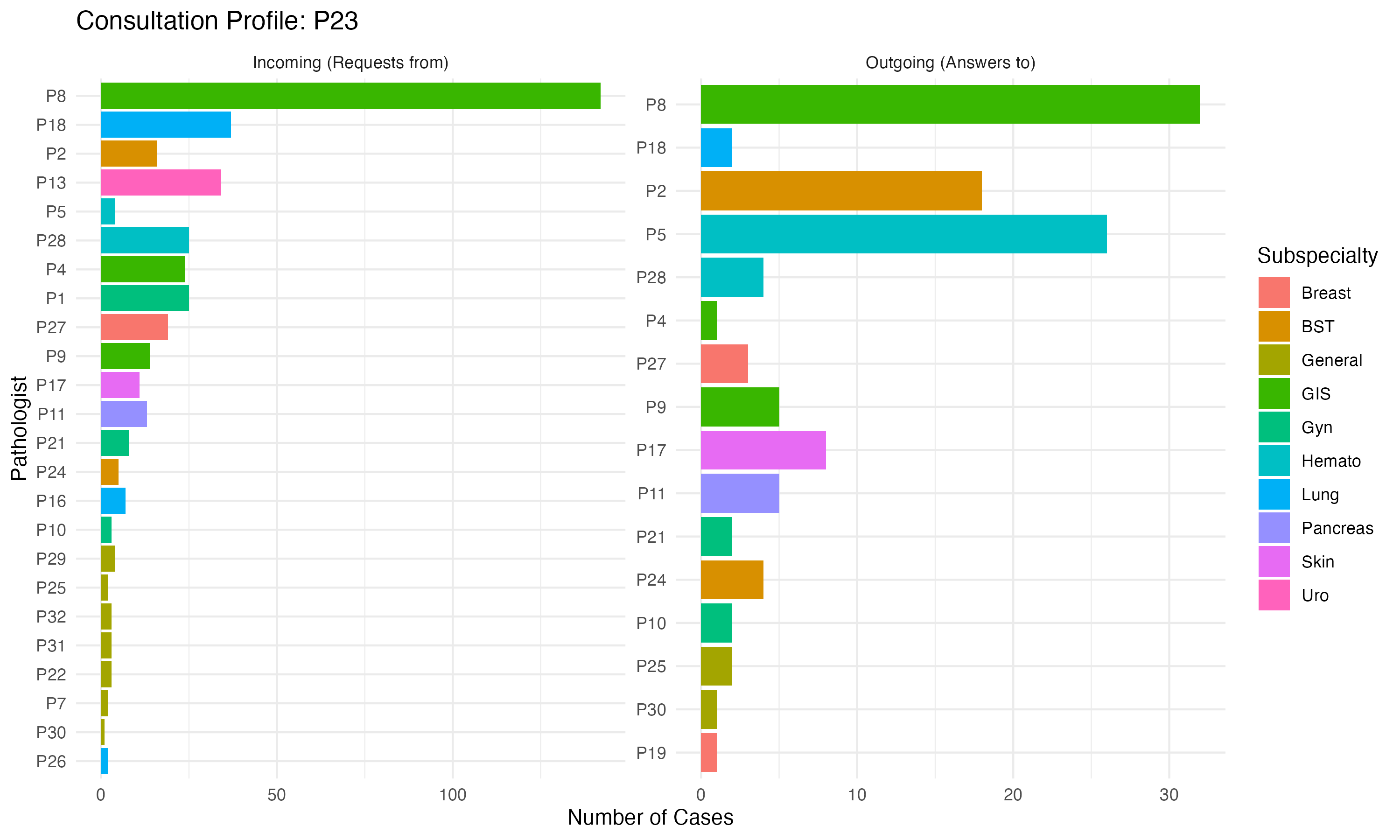
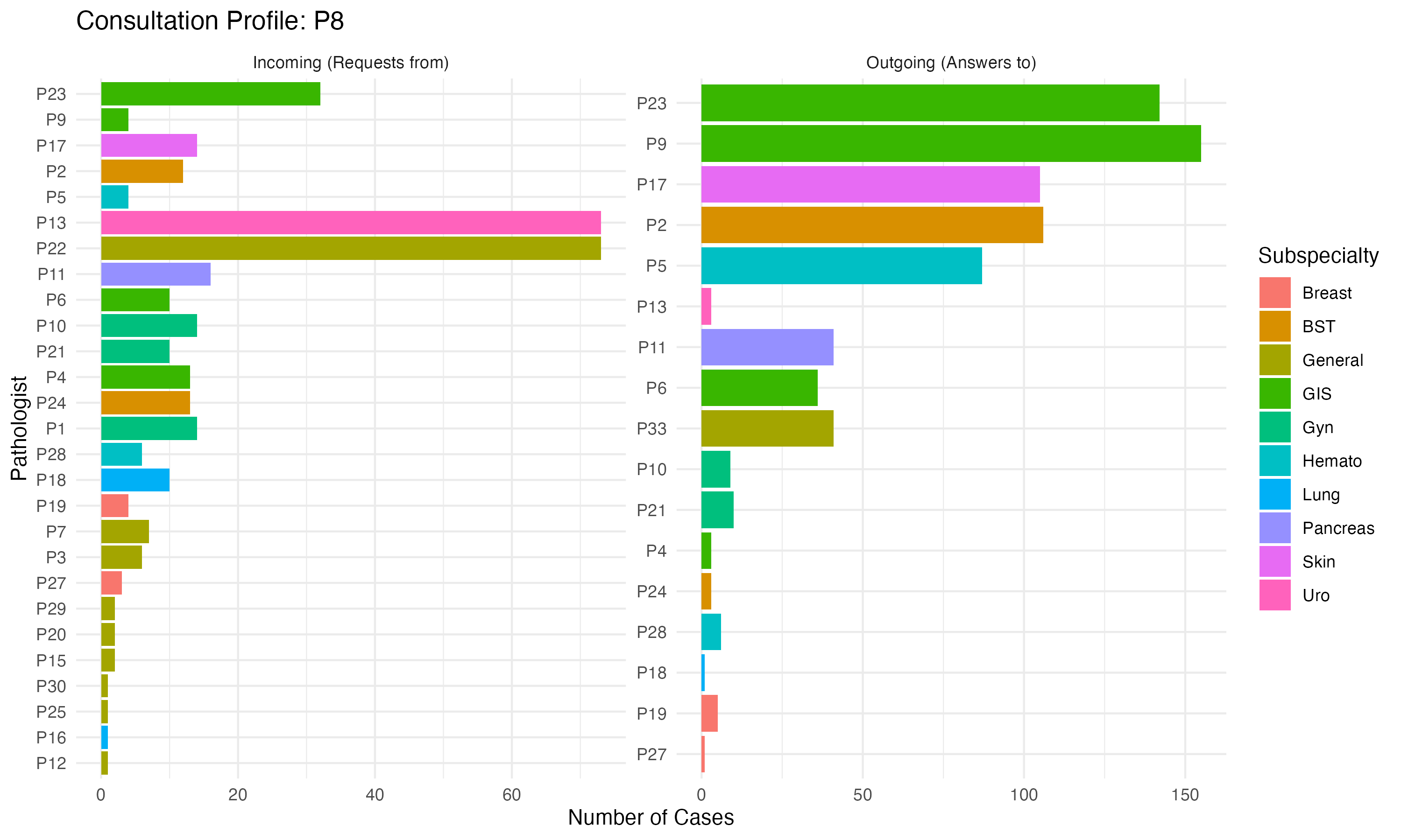
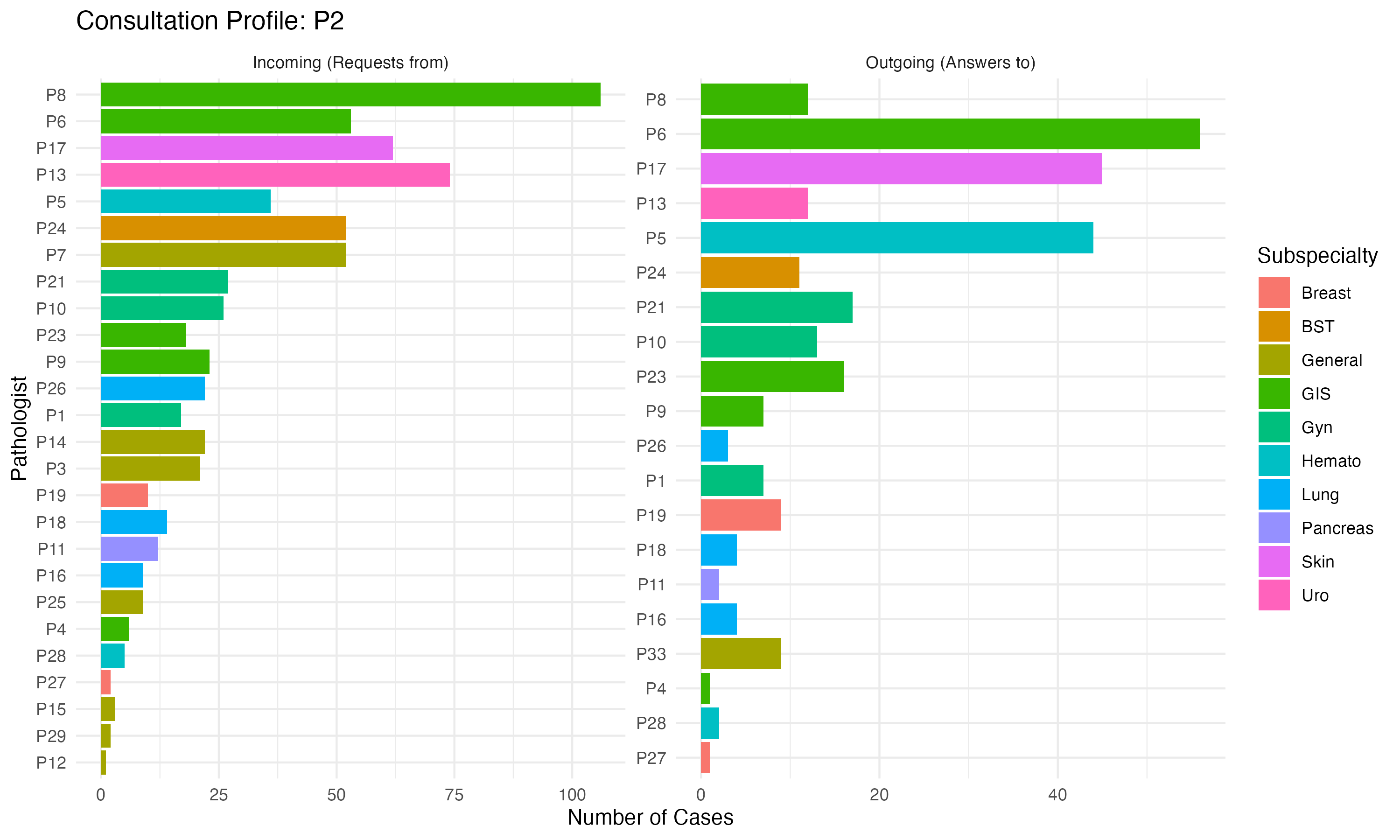
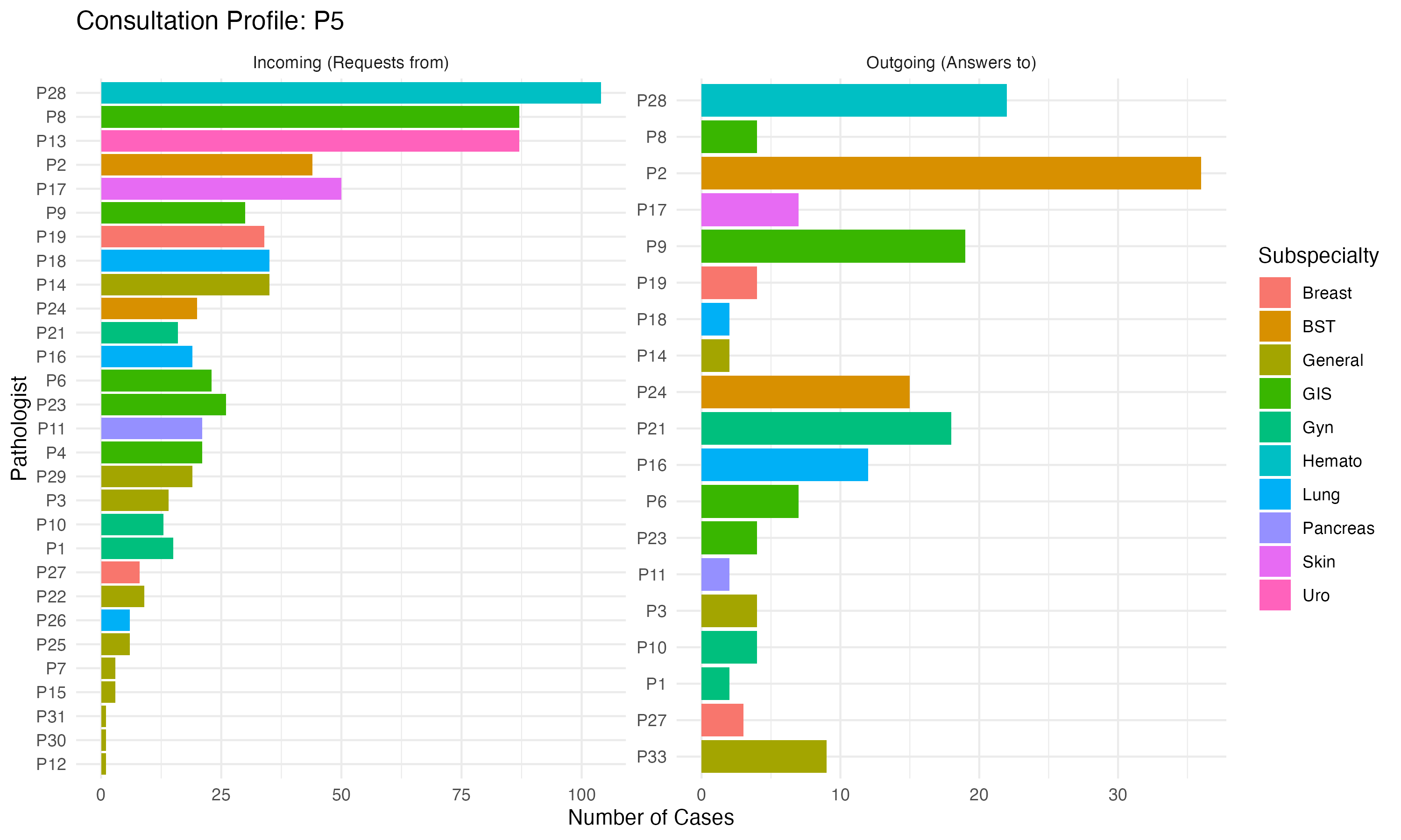
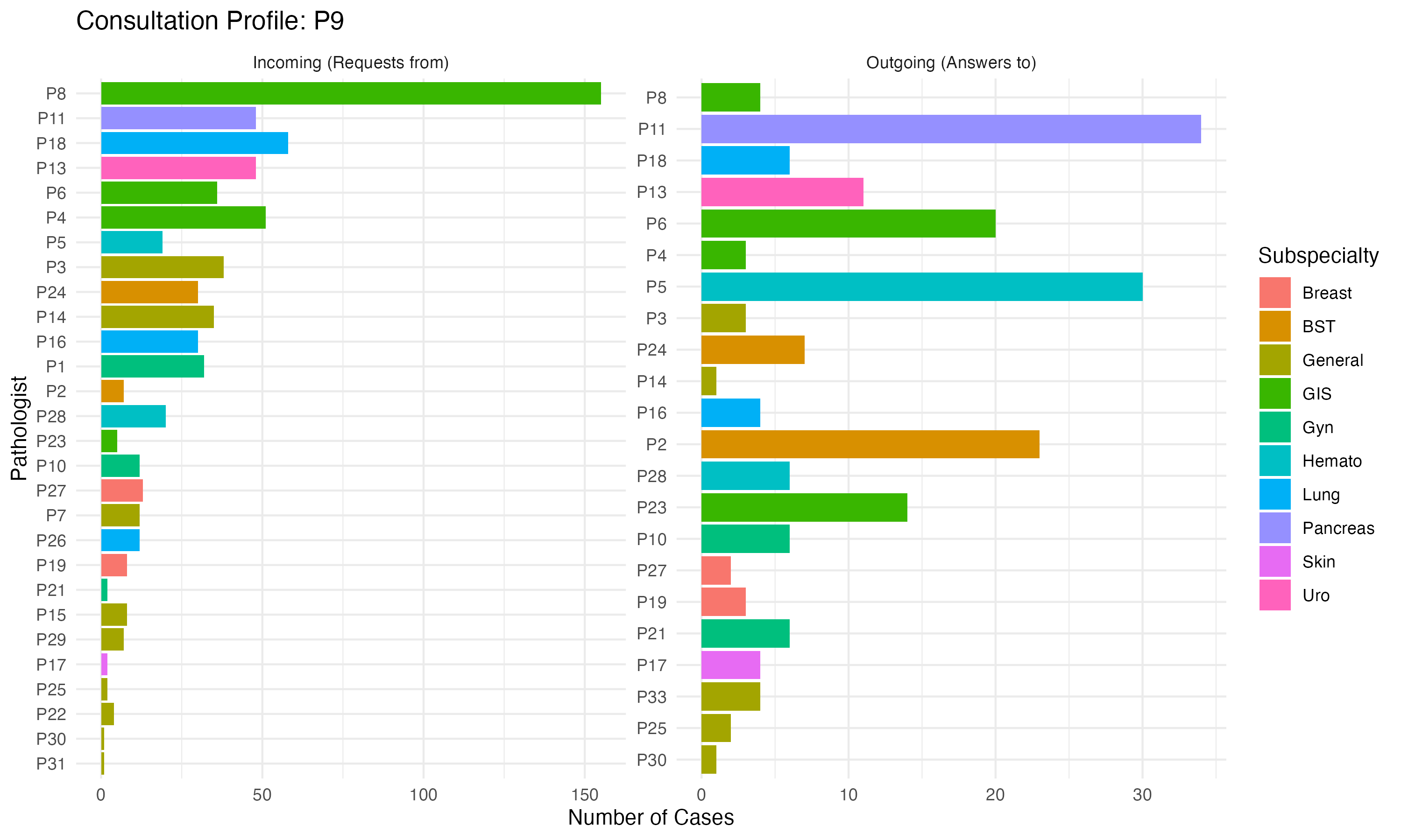
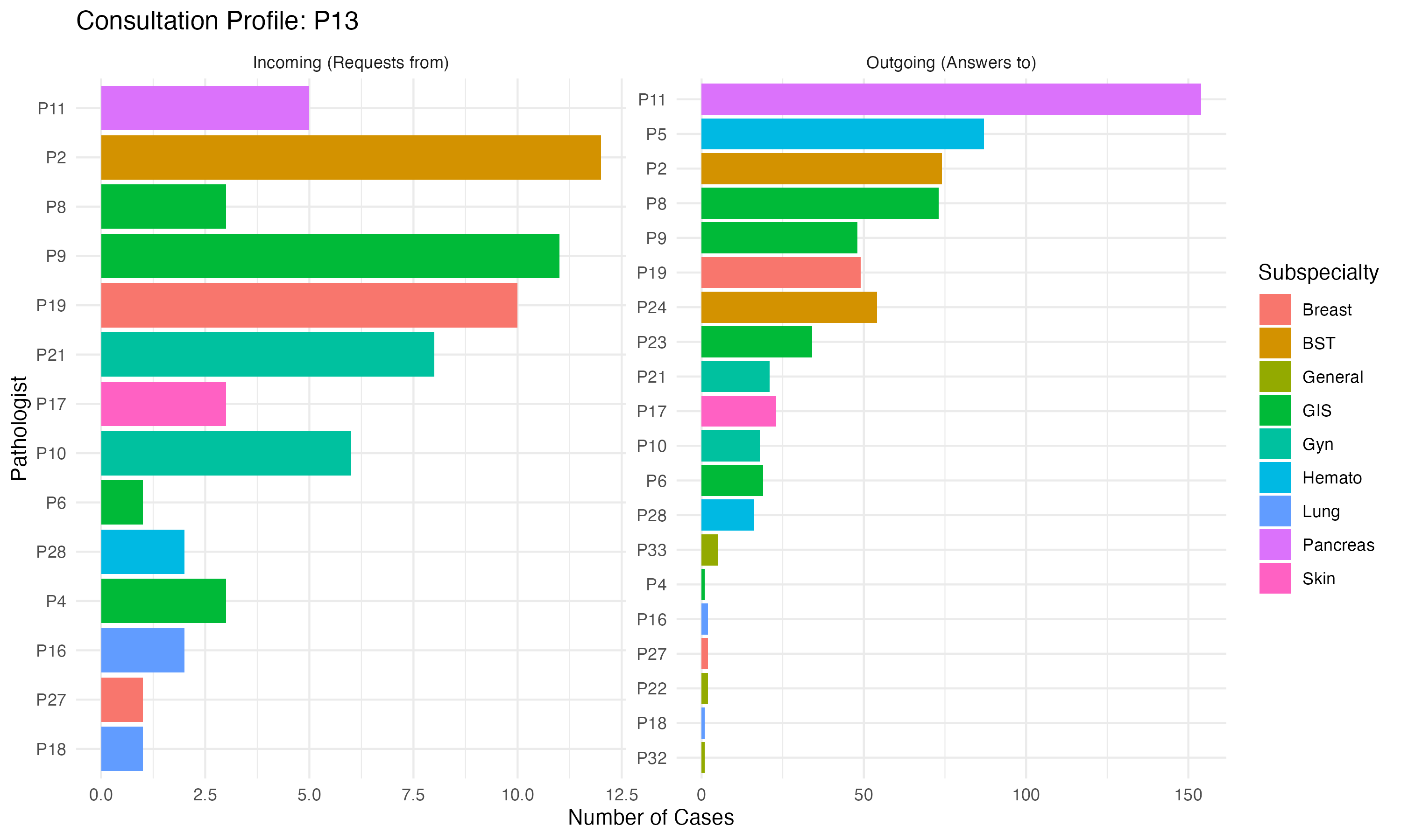
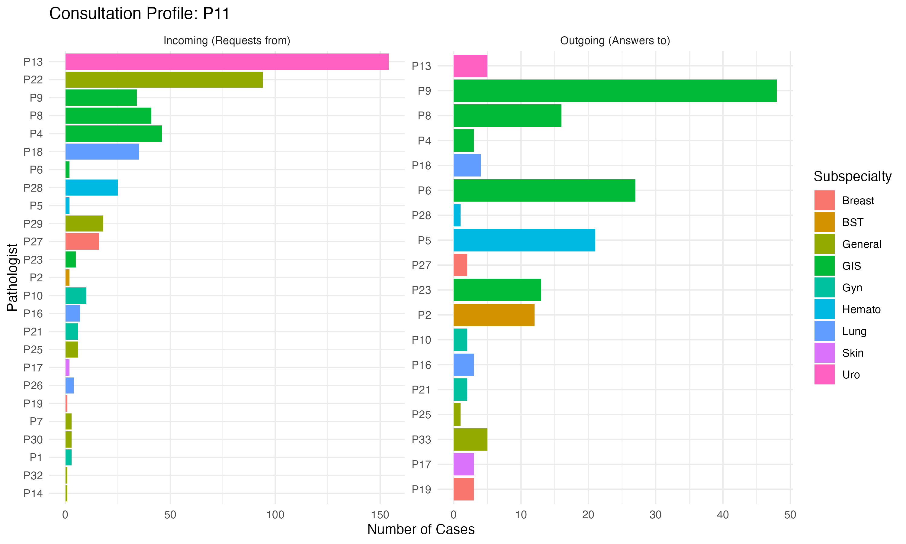
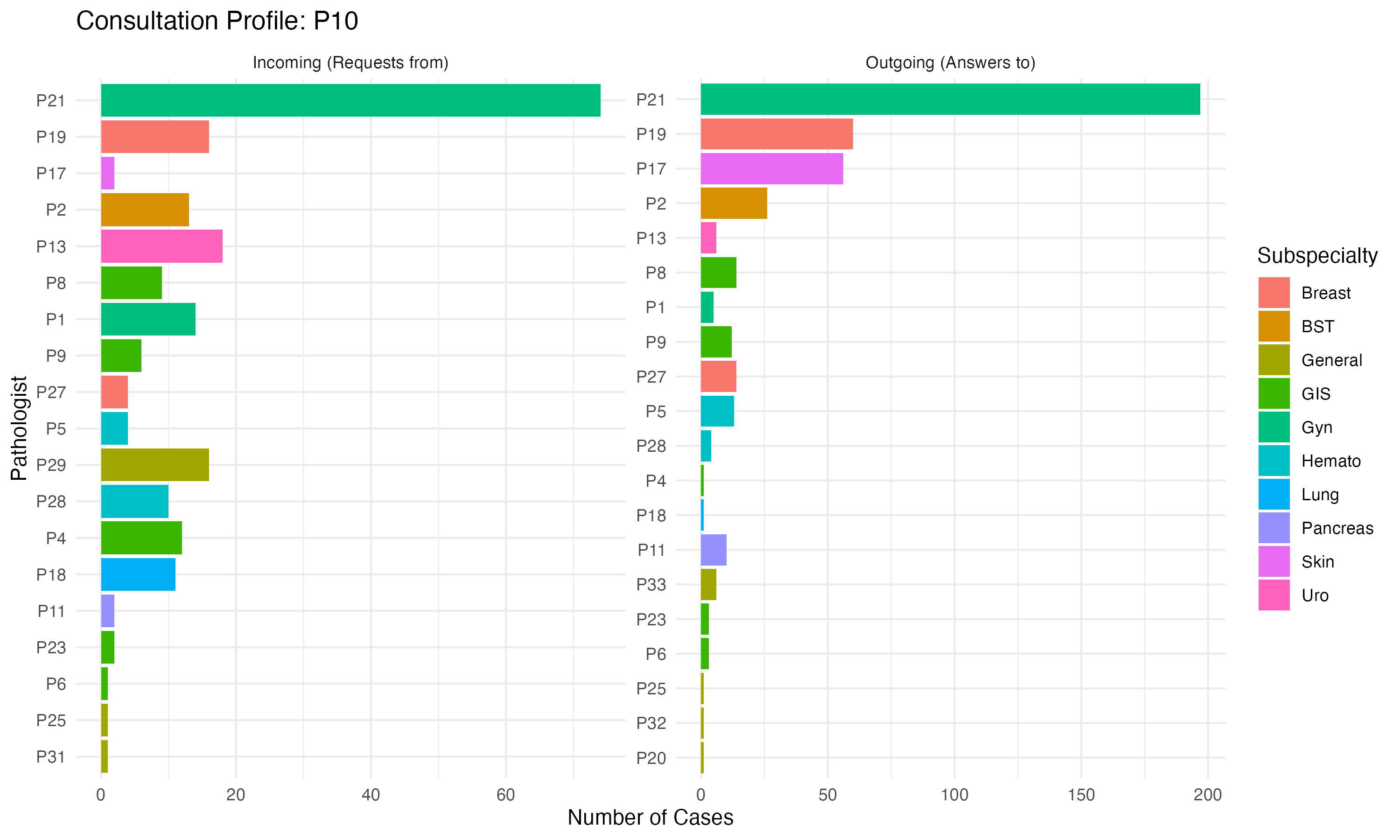
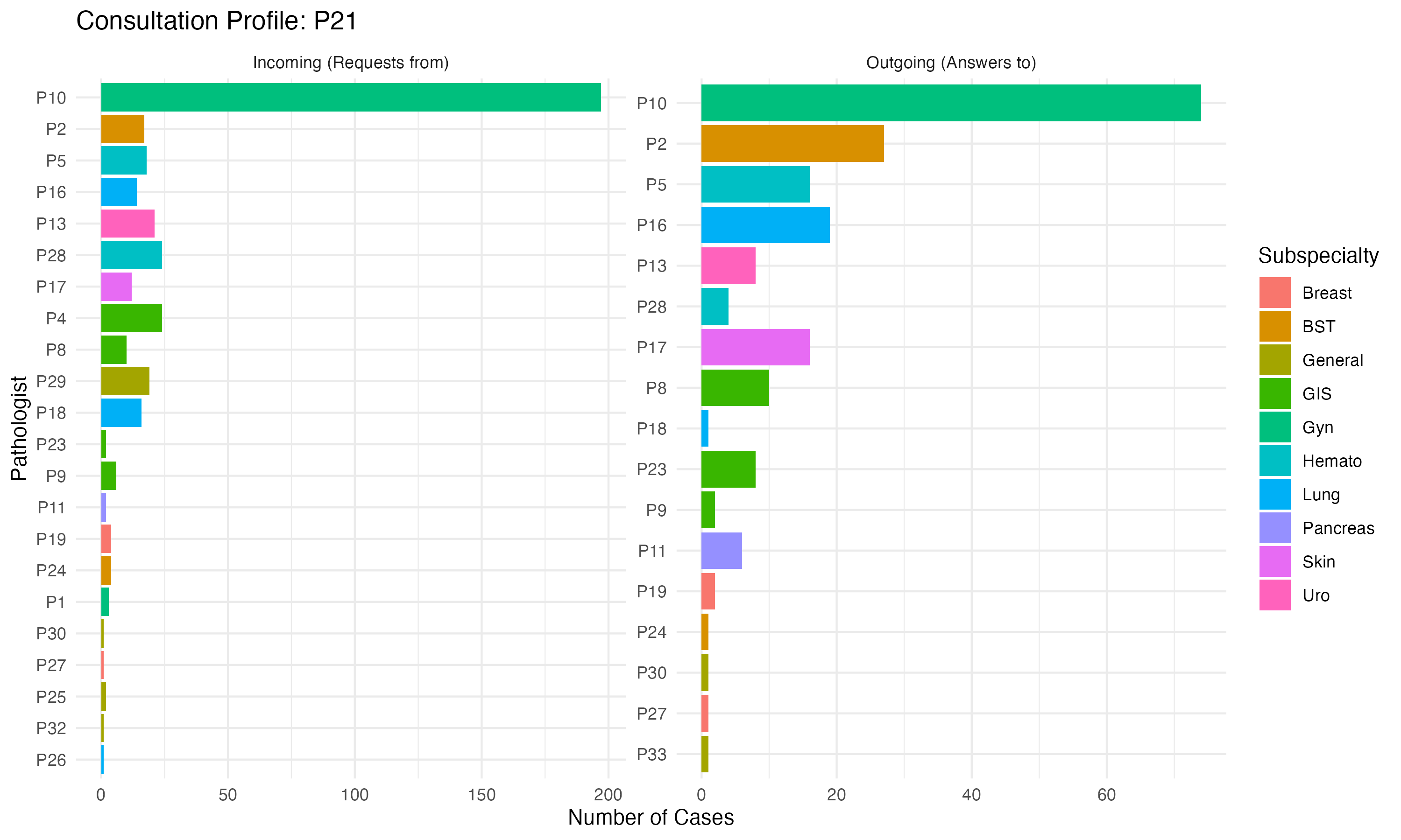
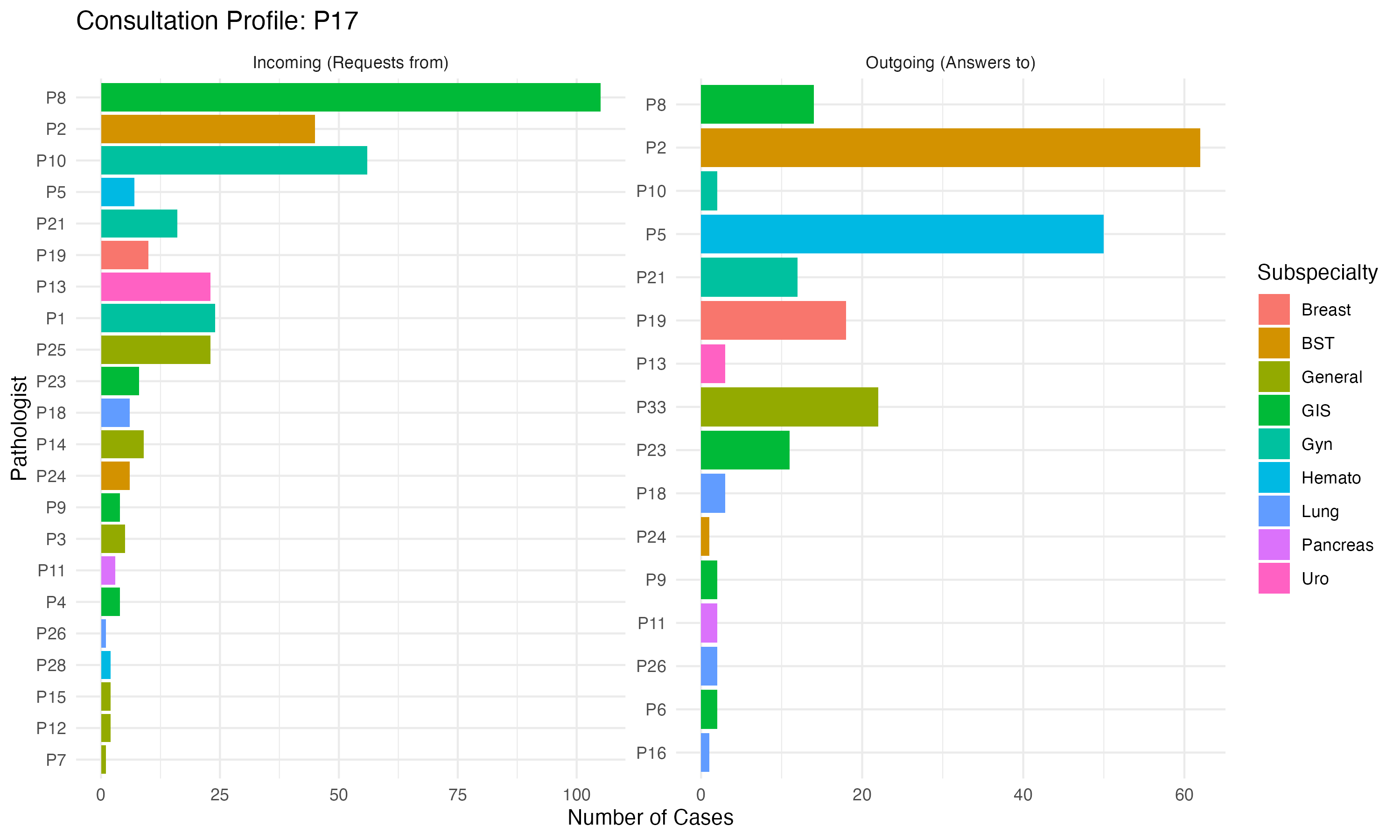
Visualizing the specific consultation patterns for key pathologists. These “Sankey” diagrams show: - Left Flows: Consultations requested BY OTHERS assigned TO the focus pathologist. - Right Flows: Consultations requested BY the focus pathologist TO OTHERS. - Colors: Based on the primary subspecialty of the connected pathologist.
9.12.1 Pathologist P8
9.12.2 Pathologist P2
9.12.3 Pathologist P5
9.12.4 Pathologist P9
9.12.5 Pathologist P13
9.12.6 Pathologist P11
9.12.7 Pathologist P10
9.12.8 Pathologist P21
9.12.9 Pathologist P17
9.12.10 Pathologist P23