[1] TRUE18 Advanced Statistical Analysis
This chapter implements advanced analytical methods identified through literature review to deepen the understanding of intradepartmental consultation patterns. Each section compares results with published benchmarks. Methods include funnel plots for institutional performance comparison (Spiegelhalter 2005), mixed-effects models for hierarchical data (Brown and Prescott 2021), change point detection for identifying process shifts (Killick and Eckley 2014), association rule mining for discovering co-occurrence patterns (Agrawal, Imieliński, and Swami 1993), and concordance analysis benchmarked against published diagnostic discordance rates (Elmore et al. 2015). Where interrupted time series methods are applied, we follow recent methodological guidance on autocorrelation adjustment, impact model specification, and segmented regression – areas where a systematic review of 120 health system QI studies found widespread deficiencies (Hategeka et al. 2020; Penfold and Zhang 2013; Bernal, Cummins, and Gasparrini 2017).
18.1 Diagnostic Concordance Analysis
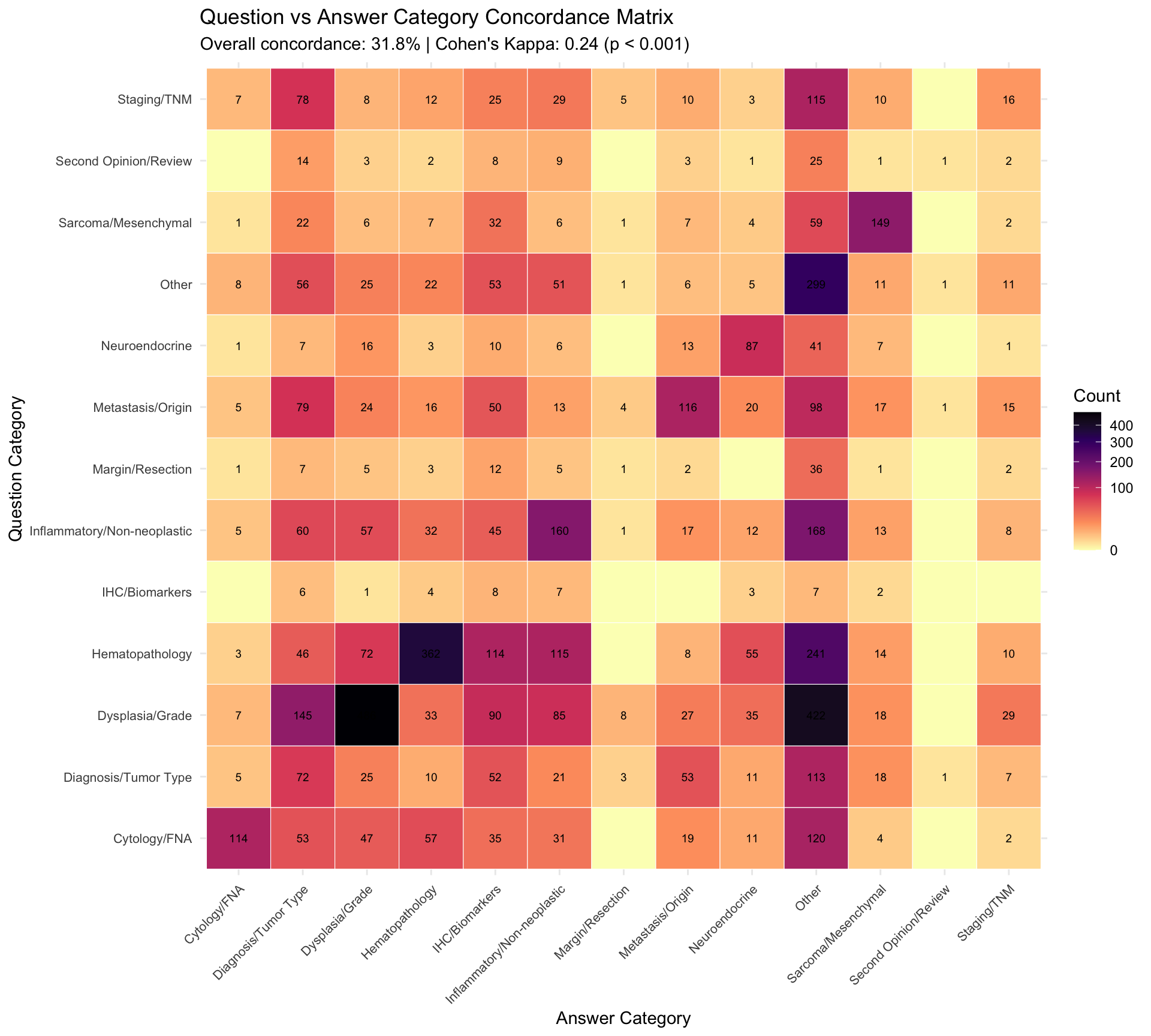
The concordance between Question_Category and Answer_Category reveals how often the responder’s diagnostic framing aligns with the asker’s initial assessment. Published discordance rates in digital pathology range from 1.7% (Azam et al. 2021) (meta-analysis of 25 studies) to 4.7% (second opinion reviews). However, category-level concordance measures a different construct: whether the type of diagnostic question shifts during consultation.
| Question Category | Total | Same | Shifted | Concordance % | Most Common Shift |
|---|---|---|---|---|---|
| Margin/Resection | 75 | 1 | 74 | 1.3 | Other (36) |
| Second Opinion/Review | 69 | 1 | 68 | 1.4 | Other (25) |
| Staging/TNM | 318 | 16 | 302 | 5.0 | Other (115) |
| Diagnosis/Tumor Type | 391 | 72 | 319 | 18.4 | Other (113) |
| IHC/Biomarkers | 38 | 8 | 30 | 21.1 | Inflammatory/Non-neoplastic (7) |
| Cytology/FNA | 493 | 114 | 379 | 23.1 | Other (120) |
| Metastasis/Origin | 458 | 116 | 342 | 25.3 | Other (98) |
| Inflammatory/Non-neoplastic | 578 | 160 | 418 | 27.7 | Other (168) |
| Hematopathology | 1040 | 362 | 678 | 34.8 | Other (241) |
| Dysplasia/Grade | 1385 | 486 | 899 | 35.1 | Other (422) |
| Neuroendocrine | 192 | 87 | 105 | 45.3 | Other (41) |
| Sarcoma/Mesenchymal | 296 | 149 | 147 | 50.3 | Other (59) |
| Other | 549 | 299 | 250 | 54.5 | Diagnosis/Tumor Type (56) |
Literature Comparison: Our overall concordance rate of 31.8% and Cohen’s Kappa of 0.24 measure category-level agreement between two automated keyword classifications of different text fields (question text vs answer text). This is a non-standard application of Cohen’s Kappa, which was originally designed for inter-rater reliability between independent human raters on the same items. Here, it serves as a chance-corrected measure of whether the algorithmic categorization of the question aligns with that of the answer. This is distinct from diagnostic concordance (98.3% reported by Azam et al. (2021)). The category shift reflects the natural evolution of a diagnostic question during consultation — the asker frames a question about dysplasia grading, but the answer addresses tumor typing. This is expected behavior in intradepartmental consultations rather than disagreement.
| Responder Seniority | N Consultations | Concordance % |
|---|---|---|
| Senior Consultant | 4365 | 33.2 |
| Junior | 313 | 32.3 |
| Consultant | 914 | 31.5 |
| SeniorConsultant | 29 | 20.7 |
18.2 Time-to-Completion Analysis (Survival Framework)
Survival analysis methods treat TAT as a time-to-event variable, providing a natural framework for modeling consultation completion times. Patel (2006) pioneered this approach for pathology TAT, and the CAP Q-Probes study (2015) identified IHC use, consultation, and malignancy as key TAT predictors.
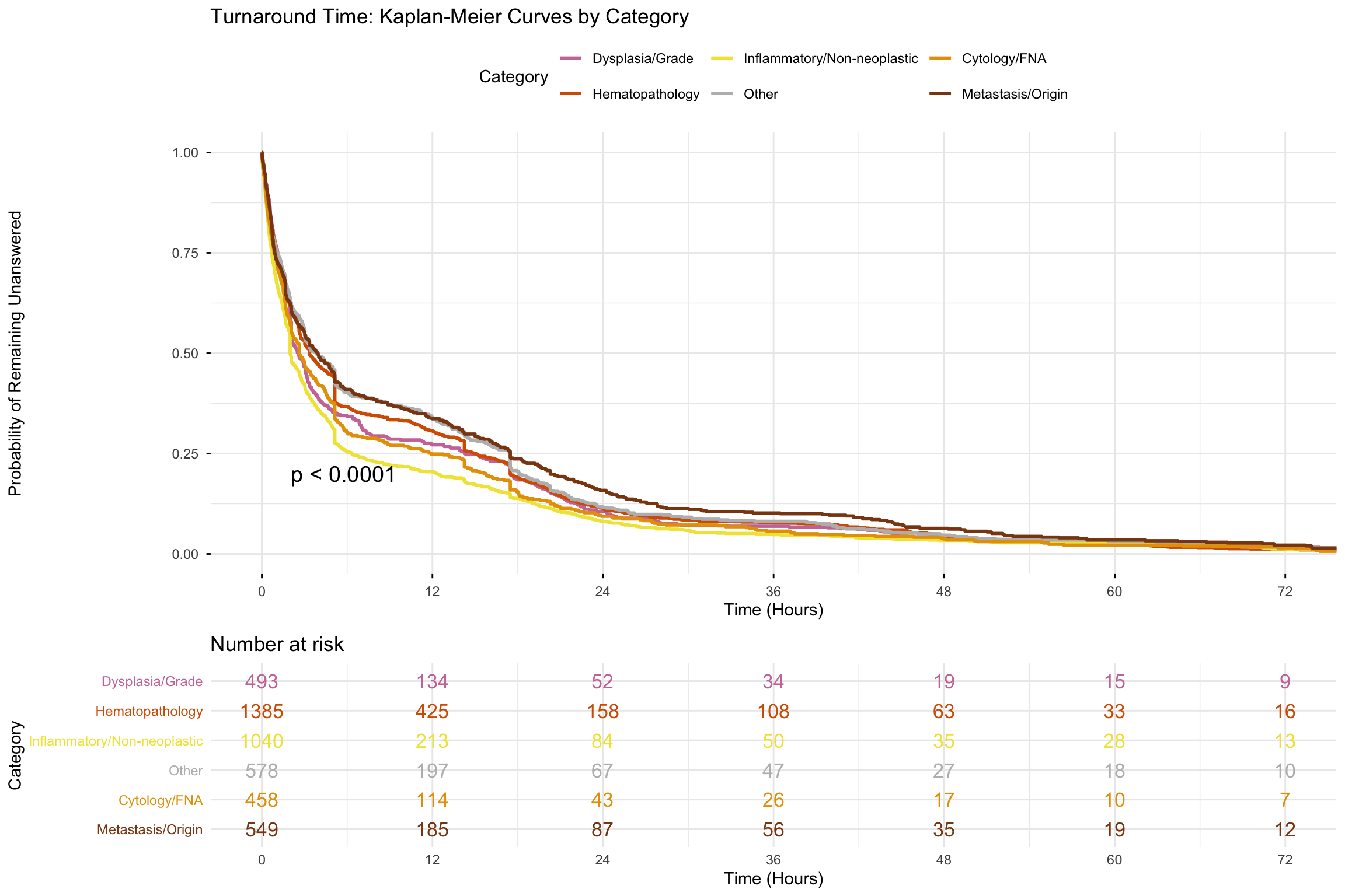
Note on censoring: Since all consultations in this dataset reached completion, there is no right-censoring — every record is an observed event. The Kaplan-Meier curves below therefore represent empirical cumulative distribution functions (1 - CDF), and the log-rank test is equivalent to a Kruskal-Wallis comparison of distributions. The survival framework is used here for its visual interpretability (probability of remaining unanswered at time t) and for the Cox proportional hazards model, which provides a convenient regression framework for comparing distributions across covariates.
18.2.1 Kaplan-Meier Curves by Category
18.2.2 Cox Proportional Hazards Model
| Term | Hazard Ratio | 95% CI Low | 95% CI High | P-value | Interpretation |
|---|---|---|---|---|---|
| Cat: Hematopathology | 1.138 | 1.020 | 1.270 | 0.021 | Faster response |
| Cat: Sarcoma/Mesenchymal | 1.066 | 0.919 | 1.237 | 0.399 | Faster response |
| Cat: Metastasis/Origin | 1.041 | 0.914 | 1.186 | 0.543 | Faster response |
| Cat: Diagnosis/Tumor Type | 1.041 | 0.908 | 1.193 | 0.564 | Faster response |
| Seniority: Junior | 1.000 | 0.879 | 1.139 | 0.994 | Faster response |
| Cat: Inflammatory/Non-neoplastic | 0.950 | 0.840 | 1.075 | 0.417 | Slower response |
| Cat: Neuroendocrine | 0.942 | 0.795 | 1.118 | 0.495 | Slower response |
| Cat: Dysplasia/Grade | 0.938 | 0.844 | 1.043 | 0.236 | Slower response |
| Cat: Second Opinion/Review | 0.924 | 0.709 | 1.205 | 0.561 | Slower response |
| Cat: Margin/Resection | 0.898 | 0.692 | 1.163 | 0.414 | Slower response |
| Is_Multi | 0.889 | 0.840 | 0.941 | 0.000 | Slower response |
| Cat: Other | 0.880 | 0.777 | 0.996 | 0.043 | Slower response |
| Cat: IHC/Biomarkers | 0.833 | 0.585 | 1.186 | 0.310 | Slower response |
| Seniority: Senior Consultant | 0.809 | 0.752 | 0.870 | 0.000 | Slower response |
| Cat: Staging/TNM | 0.775 | 0.670 | 0.897 | 0.001 | Slower response |
| Seniority: SeniorConsultant | 0.644 | 0.444 | 0.934 | 0.020 | Slower response |
| IsWeekend | 0.619 | 0.573 | 0.669 | 0.000 | Slower response |
18.2.3 Proportional Hazards Assumption Check
The Cox model assumes that hazard ratios remain constant over time. Violation of this assumption (e.g., if category effects change across the TAT range) would make the reported hazard ratios time-averaged summaries rather than true constant effects.
| Variable | Chi-sq | DF | P-value | Interpretation | |
|---|---|---|---|---|---|
| Question_Category | Question_Category | 33.033 | 12 | <0.001 | PH assumption violated -- hazard ratio is time-varying |
| Responder_Seniority | Responder_Seniority | 7.556 | 3 | 0.0561 | PH assumption satisfied |
| Is_Multi | Is_Multi | 15.712 | 1 | <0.001 | PH assumption violated -- hazard ratio is time-varying |
| IsWeekend | IsWeekend | 24.605 | 1 | <0.001 | PH assumption violated -- hazard ratio is time-varying |
| GLOBAL | GLOBAL | 77.695 | 17 | <0.001 | PH assumption violated -- hazard ratio is time-varying |
Literature Comparison: The CAP Q-Probes study (Volmar et al. 2015) found consultation with other pathologists and IHC use significantly prolonged TAT in multivariate analysis. Our Cox model quantifies these effects as hazard ratios — values < 1 indicate longer TAT (slower “resolution”). Where the proportional hazards assumption is violated, the reported hazard ratio should be interpreted as a weighted time-average rather than a constant effect.
18.3 Statistical Process Control
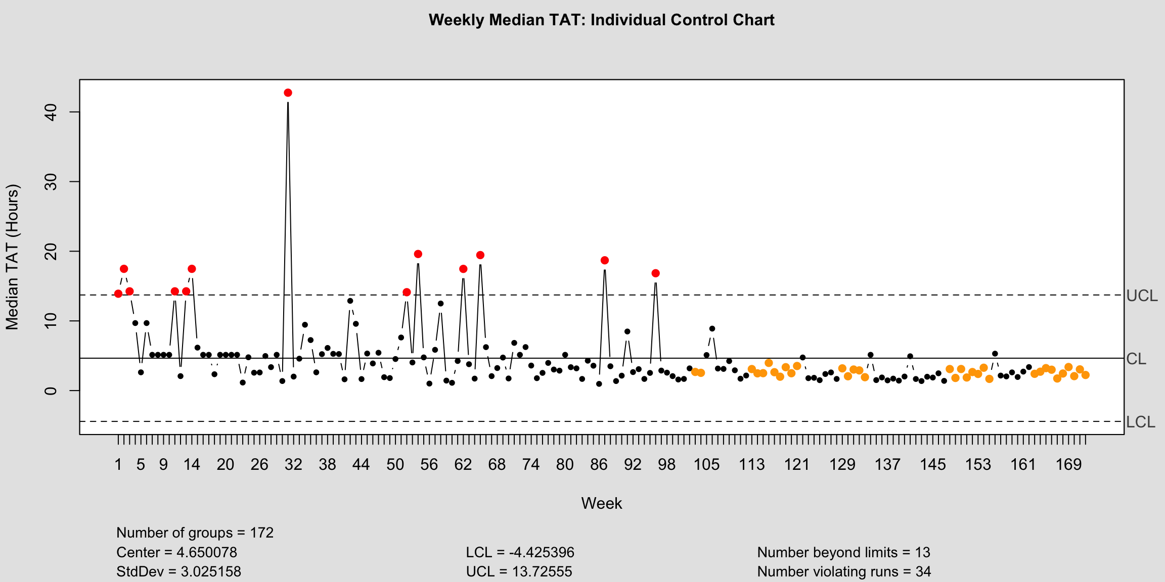
SPC charts distinguish common-cause variation (inherent to the process) from special-cause variation (something changed). This is the standard approach in laboratory quality management (Westgard and Westgard 2016).
18.3.1 TAT Control Chart
| Metric | Value |
|---|---|
| Total Weeks Analyzed | 172 |
| Center Line (Mean) | 4.65 |
| Upper Control Limit (UCL) | 13.73 |
| Lower Control Limit (LCL) | 0 |
| Out-of-Control Points | 47 |
| Process Stability | Unstable (47 violations) |
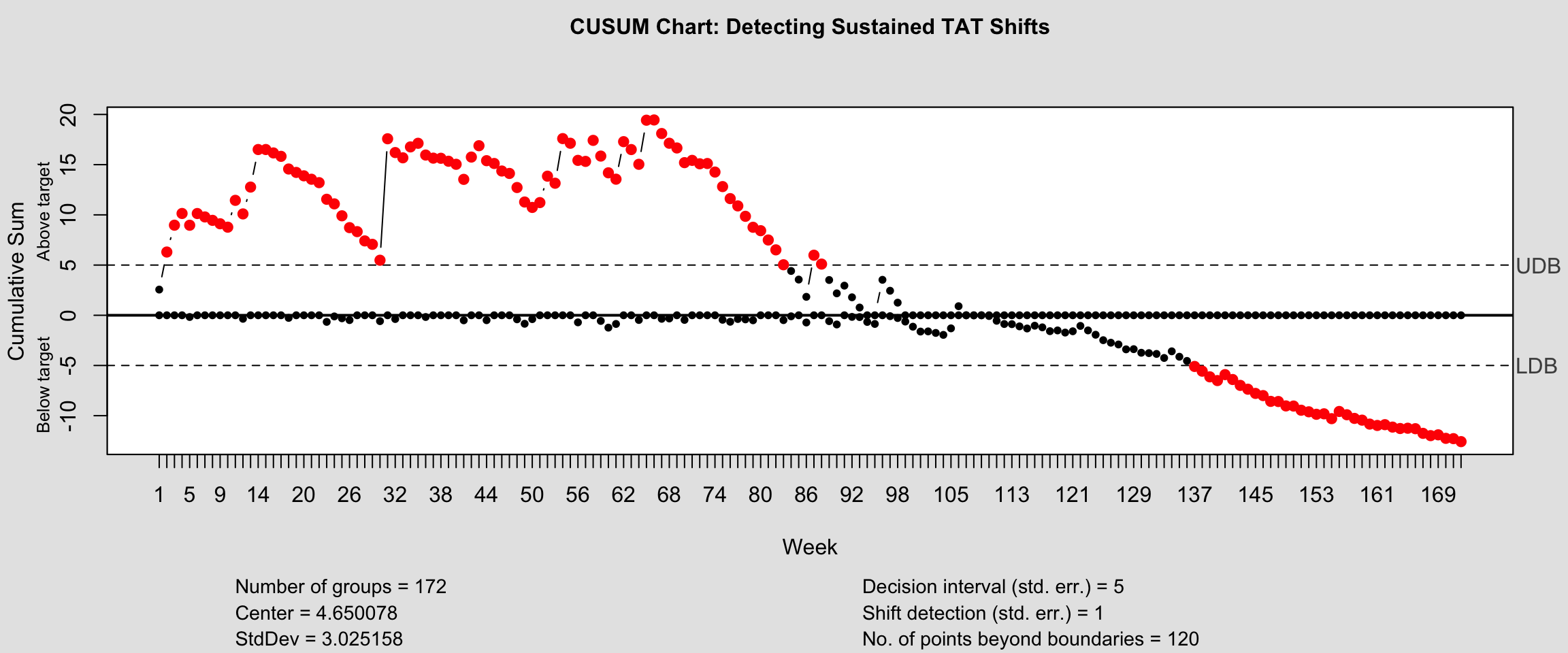
18.3.2 CUSUM Chart for TAT Drift Detection
List of 14
 $ call             : language qcc::cusum(data = weekly_tat$Median_TAT, title = "CUSUM Chart: Detecting Sustained TAT Shifts",      xlab = "Week| __truncated__
 $ type             : chr "cusum"
 $ data.name        : chr "weekly_tat$Median_TAT"
 $ data             : num [1:172, 1] 13.91 17.48 14.25 9.69 2.62 ...
  ..- attr(*, "dimnames")=List of 2
 $ statistics       : Named num [1:172] 13.91 17.48 14.25 9.69 2.62 ...
  ..- attr(*, "names")= chr [1:172] "1" "2" "3" "4" ...
 $ sizes            : int [1:172] 1 1 1 1 1 1 1 1 1 1 ...
 $ center           : num 4.65
 $ std.dev          : num 3.03
 $ pos              : num [1:172] 2.56 6.3 8.97 10.14 8.97 ...
 $ neg              : num [1:172] 0 0 0 0 -0.171 ...
 $ head.start       : num 0
 $ decision.interval: num 5
 $ se.shift         : num 1
 $ violations       :List of 2
 - attr(*, "class")= chr "cusum.qcc"
18.3.3 Consultation Volume Control Chart
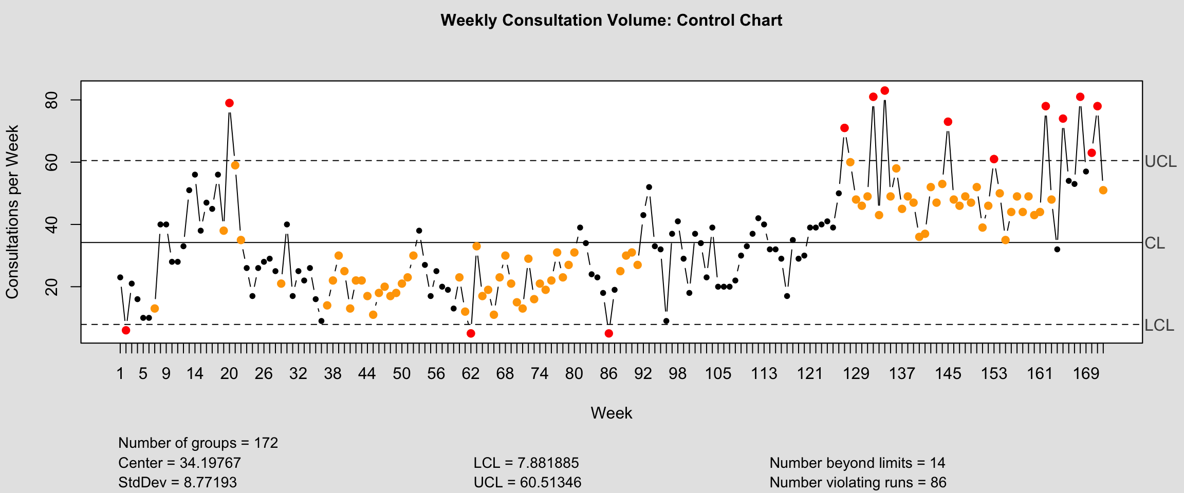
List of 11
 $ call      : language qcc::qcc(data = weekly_volume$n, type = "xbar.one", title = "Weekly Consultation Volume: Control Chart",      xla| __truncated__
 $ type      : chr "xbar.one"
 $ data.name : chr "weekly_volume$n"
 $ data      : int [1:172, 1] 23 6 21 16 10 10 13 40 40 28 ...
  ..- attr(*, "dimnames")=List of 2
 $ statistics: Named int [1:172] 23 6 21 16 10 10 13 40 40 28 ...
  ..- attr(*, "names")= chr [1:172] "1" "2" "3" "4" ...
 $ sizes     : int [1:172] 1 1 1 1 1 1 1 1 1 1 ...
 $ center    : num 34.2
 $ std.dev   : num 8.77
 $ nsigmas   : num 3
 $ limits    : num [1, 1:2] 7.88 60.51
  ..- attr(*, "dimnames")=List of 2
 $ violations:List of 2
 - attr(*, "class")= chr "qcc"
18.4 Funnel Plots for Pathologist Performance
Funnel plots compare individual pathologist TAT against volume, with control limits that account for the natural increase in variability at lower volumes. This avoids penalizing low-volume pathologists for naturally more variable metrics (Spiegelhalter 2005).
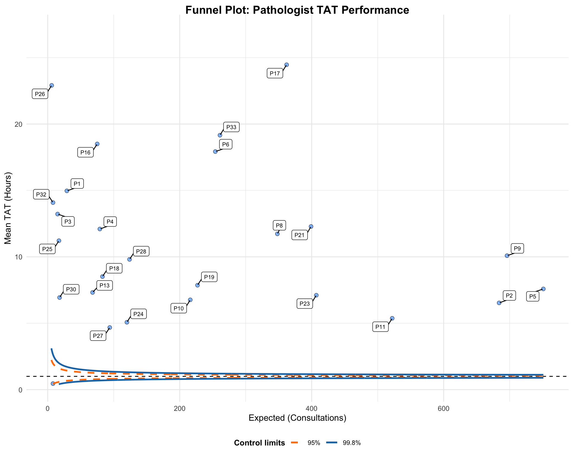
A funnel plot object with 26 points of which 25 are outliers.
Plot is not adjusted for overdispersion. | Responder | N | Mean_TAT | Expected | Z_Score | Status |
|---|---|---|---|---|---|
| P17 | 362 | 24.46 | 10.3 | 16.74 | Outside 99.8% limits |
| P33 | 261 | 19.16 | 10.3 | 8.89 | Outside 99.8% limits |
| P6 | 254 | 17.93 | 10.3 | 7.55 | Outside 99.8% limits |
| P11 | 522 | 5.37 | 10.3 | -6.99 | Outside 99.8% limits |
| P2 | 684 | 6.53 | 10.3 | -6.12 | Outside 99.8% limits |
| P5 | 751 | 7.58 | 10.3 | -4.62 | Outside 99.8% limits |
| P16 | 75 | 18.50 | 10.3 | 4.41 | Outside 99.8% limits |
| P23 | 407 | 7.11 | 10.3 | -4.00 | Outside 99.8% limits |
| P24 | 120 | 5.07 | 10.3 | -3.56 | Outside 99.8% limits |
| P27 | 94 | 4.68 | 10.3 | -3.39 | Outside 99.8% limits |
| P10 | 216 | 6.76 | 10.3 | -3.23 | Outside 99.8% limits |
| P21 | 399 | 12.29 | 10.3 | 2.46 | Outside 95% limits |
| P19 | 227 | 7.86 | 10.3 | -2.28 | Outside 95% limits |
18.5 Shannon Entropy: Specialization Index
Shannon entropy quantifies the diversity of each pathologist’s consultation portfolio. A specialist concentrating on one category has low entropy; a generalist spread across many categories has high entropy.
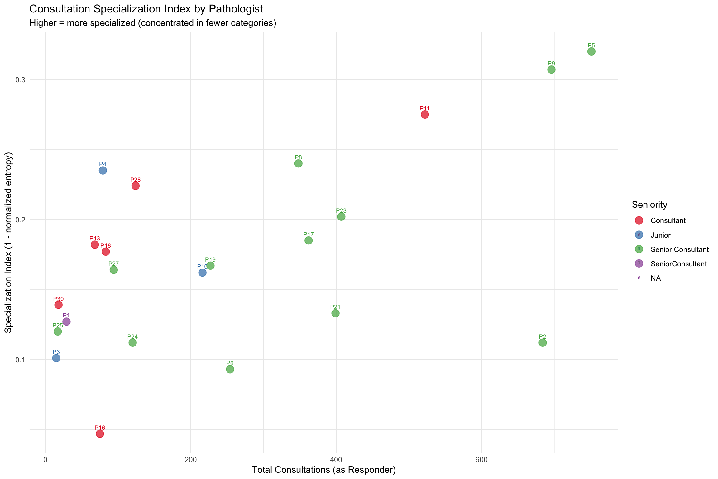
| Seniority | N Pathologists | Mean Spec. Index | SD | Avg Categories Used |
|---|---|---|---|---|
| Consultant | 6 | 0.174 | 0.078 | 10.8 |
| Junior | 3 | 0.166 | 0.067 | 10.3 |
| Senior Consultant | 12 | 0.180 | 0.076 | 12.1 |
| SeniorConsultant | 1 | 0.127 | NA | 9.0 |
| Responder | Seniority | N_Consultations | N_Categories | Specialization_Index |
|---|---|---|---|---|
| P5 | Senior Consultant | 751 | 13 | 0.320 |
| P9 | Senior Consultant | 696 | 13 | 0.307 |
| P11 | Consultant | 522 | 12 | 0.275 |
| P8 | Senior Consultant | 348 | 13 | 0.240 |
| P4 | Junior | 79 | 11 | 0.235 |
| P28 | Consultant | 124 | 12 | 0.224 |
| P23 | Senior Consultant | 407 | 13 | 0.202 |
| P17 | Senior Consultant | 362 | 13 | 0.185 |
| P13 | Consultant | 68 | 11 | 0.182 |
| P18 | Consultant | 83 | 12 | 0.177 |
18.6 Mixed-Effects Models for TAT
Standard regression ignores the hierarchical structure of our data (consultations nested within Asker-Responder pairs). Mixed-effects models partition variance between individual pathologists and case-level factors, providing more accurate estimates (Brown, 2021).
| effect | group | term | estimate | std.error | statistic | df | p.value |
|---|---|---|---|---|---|---|---|
| fixed | NA | Intercept | 1.047 | 0.253 | 4.148 | 34.766 | 0.000 |
| fixed | NA | Cat: Diagnosis/Tumor Type | -0.229 | 0.118 | -1.944 | 5270.797 | 0.052 |
| fixed | NA | Cat: Dysplasia/Grade | -0.087 | 0.094 | -0.931 | 5287.233 | 0.352 |
| fixed | NA | Cat: Hematopathology | -0.292 | 0.095 | -3.077 | 5255.985 | 0.002 |
| fixed | NA | Cat: IHC/Biomarkers | 0.459 | 0.293 | 1.570 | 5572.580 | 0.116 |
| fixed | NA | Cat: Inflammatory/Non-neoplastic | -0.186 | 0.107 | -1.739 | 5315.159 | 0.082 |
| fixed | NA | Cat: Margin/Resection | 0.037 | 0.218 | 0.170 | 5463.961 | 0.865 |
| fixed | NA | Cat: Metastasis/Origin | -0.220 | 0.113 | -1.937 | 5292.279 | 0.053 |
| fixed | NA | Cat: Neuroendocrine | -0.090 | 0.145 | -0.620 | 5410.888 | 0.536 |
| fixed | NA | Cat: Other | -0.136 | 0.107 | -1.276 | 5329.642 | 0.202 |
| fixed | NA | Cat: Sarcoma/Mesenchymal | -0.154 | 0.127 | -1.212 | 5300.705 | 0.226 |
| fixed | NA | Cat: Second Opinion/Review | -0.242 | 0.222 | -1.092 | 5543.612 | 0.275 |
| fixed | NA | Cat: Staging/TNM | -0.040 | 0.128 | -0.315 | 5325.302 | 0.753 |
| fixed | NA | Seniority: Junior | 0.044 | 0.441 | 0.099 | 27.010 | 0.922 |
| fixed | NA | Seniority: Senior Consultant | 0.099 | 0.301 | 0.330 | 23.038 | 0.745 |
| fixed | NA | Seniority: SeniorConsultant | 0.734 | 0.752 | 0.975 | 24.919 | 0.339 |
| fixed | NA | IsWeekend | 0.754 | 0.064 | 11.824 | 5577.905 | 0.000 |
| fixed | NA | Repeat Event | 0.084 | 0.180 | 0.466 | 5577.459 | 0.641 |
| ran_pars | Asker | SD: Intercept | 0.228 | NA | NA | NA | NA |
| ran_pars | Responder | SD: Intercept | 0.645 | NA | NA | NA | NA |
| ran_pars | Residual | SD: Observation | 1.606 | NA | NA | NA | NA |
| Component | Variance | % of Total |
|---|---|---|
| Asker | 0.052 | 1.7 |
| Responder | 0.416 | 13.7 |
| Residual | 2.579 | 84.6 |
Interpretation: The variance decomposition shows what fraction of TAT variability is attributable to individual Asker differences, individual Responder differences, and case-level residual variation. High Responder variance indicates that who answers the consultation matters more than what the question is about.
18.7 Workload Inequality: Robin Hood Index
The Robin Hood Index (also called the Hoover Index) expresses the percentage of total workload that would need to be redistributed from above-average to below-average pathologists to achieve perfect equality. It is more intuitive than the Gini coefficient for administrators (Bonert et al. 2022).
| Metric | Value | Interpretation |
|---|---|---|
| Gini Coefficient | 0.621 | 0 = perfect equality, 1 = one pathologist does everything |
| Robin Hood Index | 0.497 | 49.7% of consultations need redistribution for equality |
| Theil Index | 0.690 | Information-theoretic inequality; 0 = equal, higher = more unequal |
Literature Comparison: Bonert et al. (2022) reported Gini coefficients of 0.05-0.23 across hospital pathology groups using L4E workload units. Our Gini of 0.621 for consultation workload specifically may differ because consultations represent a specialized subset of total pathology work. The Robin Hood Index of 49.7% quantifies the practical redistribution needed.
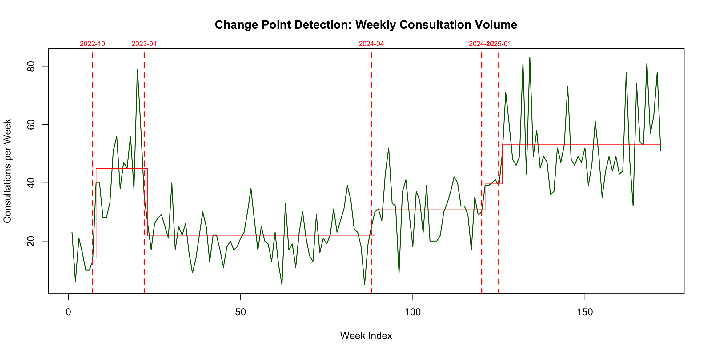
18.8 Change Point Detection
Change point analysis identifies abrupt shifts in consultation volume or TAT that may correspond to personnel changes, policy updates, or system implementations (Killick and Eckley 2014).
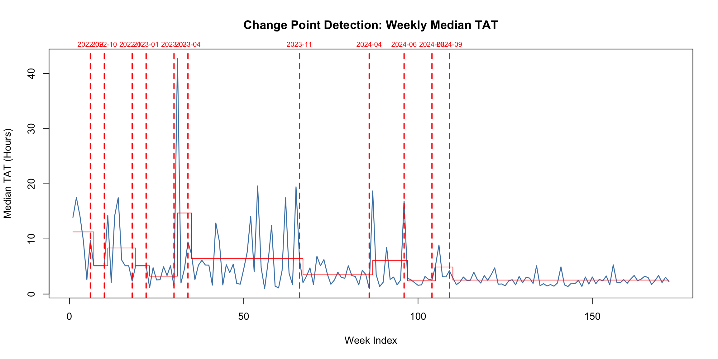
| Segment | Start_Date | End_Date | Mean_TAT | Weeks |
|---|---|---|---|---|
| 1 | 2022-08-21 | 2022-09-25 | 11.3 | 6 |
| 2 | 2022-10-02 | 2022-10-23 | 5.1 | 4 |
| 3 | 2022-10-30 | 2022-12-18 | 8.4 | 8 |
| 4 | 2022-12-25 | 2023-01-15 | 5.1 | 4 |
| 5 | 2023-01-22 | 2023-03-12 | 3.2 | 8 |
| 6 | 2023-03-19 | 2023-04-09 | 14.7 | 4 |
| 7 | 2023-04-16 | 2023-11-19 | 6.4 | 32 |
| 8 | 2023-11-26 | 2024-04-07 | 3.5 | 20 |
| 9 | 2024-04-14 | 2024-06-16 | 6.1 | 10 |
| 10 | 2024-06-23 | 2024-08-11 | 2.4 | 8 |
| 11 | 2024-08-18 | 2024-09-15 | 4.9 | 5 |
| 12 | 2024-09-22 | 2025-11-30 | 2.5 | 63 |
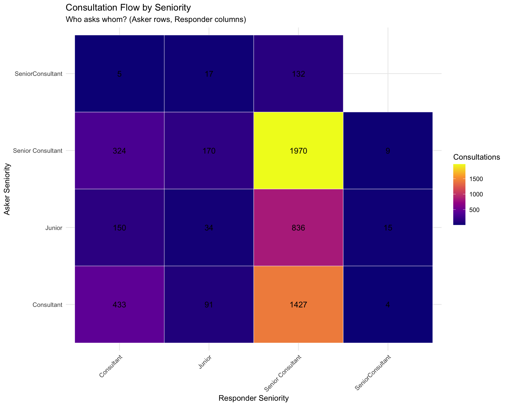
18.9 Seniority and Mentorship Analysis
Seniority-based consultation patterns reveal knowledge flow direction and potential mentorship relationships. Published literature suggests junior-to-senior consultation flow dominates in academic settings (Annals of Diagnostic Pathology, 2018).
| Direction | Count | Percentage |
|---|---|---|
| Direction | N | Median_TAT | Mean_TAT | IQR_TAT |
|---|---|---|---|---|
18.10 Network Topology: Assortativity and Core-Periphery
Advanced network metrics characterize the consultation network’s structural properties. An et al. (2018) found strong negative degree assortativity in US physician referral networks, indicating that highly-connected physicians tend to connect with less-connected ones.
| Metric | Value | Comparison |
|---|---|---|
| Degree Assortativity | -0.2285 | Disassortative (like US referral networks: -0.56) |
| Reciprocity | 0.6885 | 68.8% of edges reciprocated |
| Global Clustering Coefficient | 0.7265 | Clustering 1.3x random expectation |
| Network Density | 0.4347 | 43.5% of possible edges exist |
| Average Path Length | 2.1780 | Vs random expectation: 1.1 |
| Small-World Sigma (>1 = small-world) | 0.6151 | Not small-world |
18.10.1 Triad Census
The triad census enumerates all 16 types of directed triads, revealing whether consultation patterns form chains, cycles, or isolated pairs (An et al., 2018).
| Triad_Type | Count | Description |
|---|---|---|
| 012 | 959 | Single edge |
| 003 | 713 | Empty (no edges) |
| 111D | 692 | Mixed (1 mutual + 1 asymmetric) |
| 102 | 662 | Mutual edge |
| 300 | 528 | Complete (all mutual) |
| 210 | 345 | Near-complete |
| 201 | 290 | Two mutual pairs |
| 120D | 278 | Mixed transitivity |
| 021U | 273 | In-star |
| 111U | 223 | Mixed (1 mutual + 1 asymmetric) |
| 030T | 123 | Transitive |
| 120U | 115 | Mixed transitivity |
| 021C | 112 | Chain |
| 120C | 74 | Mixed transitivity |
| 021D | 66 | Out-star |
| 030C | 3 | Cycle |
18.11 Pareto Analysis
The Pareto Principle (80/20 rule) has been validated in surgical pathology specimen-diagnosis profiles (AJCP, 2015). We test whether it applies to consultation categories.
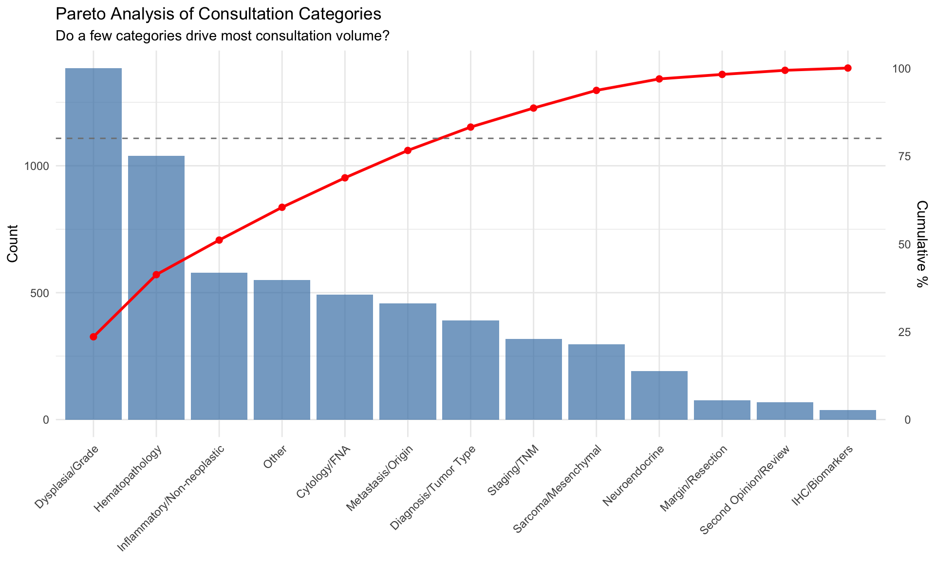
**Pareto Finding:** 7 out of 13 categories (54%) account for 80% of consultation volume.18.12 Inter-Rater Reliability (Multi-Consultant Cases)
For cases with multiple respondents, we can assess inter-rater reliability on answer categorization.
| Metric | Value |
|---|---|
| Multi-consultant cases (2 responders) | 604 |
| Raw agreement rate | 41.9% |
| Cohen's Kappa | 0.292 |
| P-value | <2e-16 |
18.13 Association Rule Mining
Association rules discover frequent co-occurrence patterns in multi-label consultation tags (Agrawal, Imieliński, and Swami 1993).
| Rule | Support | Confidence | Lift | Count | |
|---|---|---|---|---|---|
| 34 | {Metastasis/Origin,Staging/TNM} => {Margin/Resection} | 0.069 | 0.738 | 3.54 | 298 |
| 33 | {Margin/Resection,Metastasis/Origin} => {Staging/TNM} | 0.069 | 0.931 | 3.43 | 298 |
| 38 | {Inflammatory/Non-neoplastic,Metastasis/Origin} => {Margin/Resection} | 0.056 | 0.668 | 3.20 | 241 |
| 55 | {Inflammatory/Non-neoplastic,Margin/Resection} => {Staging/TNM} | 0.106 | 0.845 | 3.11 | 457 |
| 58 | {Diagnosis/Tumor Type,Margin/Resection} => {Staging/TNM} | 0.147 | 0.810 | 2.99 | 633 |
| 36 | {Dysplasia/Grade,Metastasis/Origin} => {Margin/Resection} | 0.061 | 0.620 | 2.97 | 263 |
| 53 | {Dysplasia/Grade,Staging/TNM} => {Margin/Resection} | 0.100 | 0.613 | 2.94 | 430 |
| 59 | {Diagnosis/Tumor Type,Staging/TNM} => {Margin/Resection} | 0.147 | 0.607 | 2.91 | 633 |
| 56 | {Inflammatory/Non-neoplastic,Staging/TNM} => {Margin/Resection} | 0.106 | 0.607 | 2.91 | 457 |
| 41 | {Dysplasia/Grade,Metastasis/Origin} => {Staging/TNM} | 0.077 | 0.778 | 2.87 | 330 |
| 43 | {Inflammatory/Non-neoplastic,Metastasis/Origin} => {Staging/TNM} | 0.064 | 0.765 | 2.82 | 276 |
| 52 | {Dysplasia/Grade,Margin/Resection} => {Staging/TNM} | 0.100 | 0.739 | 2.72 | 430 |
| 13 | {Staging/TNM} => {Margin/Resection} | 0.153 | 0.563 | 2.70 | 656 |
| 12 | {Margin/Resection} => {Staging/TNM} | 0.153 | 0.732 | 2.70 | 656 |
| 45 | {Diagnosis/Tumor Type,Metastasis/Origin} => {Staging/TNM} | 0.094 | 0.541 | 1.99 | 402 |
Interpretation: Rules with high lift (>>1) indicate tag pairs that co-occur much more frequently than expected by chance. These reveal tightly coupled diagnostic concepts in pathology consultations.
18.14 Summary of Advanced Analyses
| Analysis | Key Finding | Literature Benchmark |
|---|---|---|
| Concordance (Q vs A Category) | Kappa = 0.24; 31.8% concordance | Digital pathology concordance: 98.3% (Azam et al. 2021); ours measures category shift, not diagnostic error |
| Survival Analysis (Cox PH) | Cox model identifies category and seniority effects on TAT | CAP Q-Probes: IHC/consultation/malignancy prolong TAT (Volmar et al. 2015) |
| SPC Control Charts | Control chart: 47 out-of-control weeks | Westgard rules for lab quality; first application to consultation TAT (Westgard 2016) |
| Funnel Plots | 13 pathologists outside control limits | Spiegelhalter 2005: funnel plots for institutional performance comparison |
| Shannon Entropy (Specialization) | Specialization index range: 0.05 - 0.32 | Novel application; no direct pathology precedent |
| Mixed-Effects Models | Responder random effect explains 13.7% of TAT variance | Brown & Prescott 2021: mixed-effects for clustered biomedical data |
| Robin Hood Index | Robin Hood Index = 49.7% redistribution needed | Bonert et al. 2022: Gini 0.05-0.23 in pathology workload |
| Change Point Detection | 11 TAT change points, 5 volume change points | Killick & Eckley 2014: PELT algorithm for changepoint detection |
| Seniority Flow Analysis | % Junior-to-Senior flow | Goebel et al. 2018: expertise drives consultant choice in pathology |
| Network Topology (Assortativity) | Assortativity = -0.229; Small-world sigma = 0.62 | Social network analysis methods applied to physician referral networks |
| Triad Census | Dominant triad: 012 (Single edge) | Triad census analysis for understanding consultation network structure |
| Pareto Analysis | 7/13 categories cover 80% of volume | Pareto principle validated in surgical pathology case distributions |
| Inter-Rater Reliability | 839 multi-consultant cases analyzed | McHugh 2012: kappa interpretation guidelines |
| Association Rule Mining | 73 association rules discovered (support >= 5%) | Agrawal et al. 1993: association rule mining; novel application to pathology tags |